


My family went on a cruise last Christmas and we somehow found ourselves discussing how many miles it takes for a cruise boat to come to a stop. The physics on this isn't too bad, so I worked it out over dinner.

(See also: my planning notes.)
On October 14–15, 2026, I went back to Tomales Bay with a group of friends for another overnight paddle. Unlike on my previous trips, this time we only had a single car. No matter: the six rachet straps I'd brought held them all on.
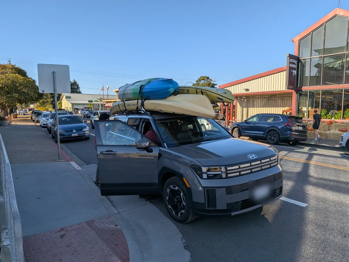
I was driving a Hyundai Santa Fe, which nominally has room for seven people. With five of us plus gear, the car was pretty packed! I'm glad I opted for the larger vehicle. Despite all the gear, we were still able to get everything on the kayaks with minimal trouble. This was aided by having 100' of paracord and a bunch of 55 gallon garbage bags to keep the stuff dry, as well as the legs of the folks in the open-deck kayaks.

The morning of the 2026 solar eclipse I stood in a room full of friends and strangers while someone tried to wrangle cars. "Who here has seen a solar eclipse?" he asked. A bunch of hands went up. "And who thinks it was the coolest thing they've ever witnessed in their entire life?" The hands stayed up. "I would recommend for your life that you go --- you won't know any different --- but the other path is better."
The other path is better. I hope you see an eclipse.
There are 124 total and hybrid solar eclipses between now and the end of 2200 offering just over seven hours of eclipse time. You won't get it all. Sometimes the shadow of the eclipse falls on Antarctica or the open ocean, or in a country known for its violence and inaccessibility to outsiders. More importantly, you'll (likely) be dead for most of the eclipse.
So, how much time do you have?
I sent one of my Prius fobs through the laundry a few years back and, ever after, the electronics just didn't work.
Recently I bought a replacement fob from Amazon, and I'm pleased to report it worked brilliantly... after I completed the chicken dance, which I'm copying from here, for posterity.
Some Prius keys have SKS. Your key has this ability if you can drive the car with the fob in your purse or pocket, not in the dash slot.
Procedure A: Programming the fob to start/stop the engine from the key port
All new fobs should be programmed for this. This will program the fob to start/stop engine while it is inserted into the key port.
- Get into the car.
- Close and unlock all doors.
- Ensure the car is off.
- Insert and remove your old fob (the one that currently works) into the fob slot 4 times in a row fairly quickly.
- Insert it a fifth and final time and leave it there.
- Open and close driver door 6 times fairly quickly.
- Remove old fob from slot.
The car should be in programming mode now. This will be indicated by the red car-shaped dash light staying on and not blinking.
If the red car-shaped dash light is not on solid, you have failed. Go back to step one and try again. Maybe you need to go faster or slower.
If the red car-shaped dash light is on solid, proceed.
- Insert your new fob and leave it in the slot. The red anti-theft light on the dashboard should begin blinking.
- When the light stops blinking and goes dark, your new fob is programmed. This may take up to a full minute.
- Remove the new fob.
You're now done with the START/STOP portion of the programming.
If you have SKS, proceed to PROCEDURE B don't have SKS, proceed to PROCEDURE C).
Procedure B: Locking/unlocking doors + smart key functionality, if you have SKS
This procedure is for chrome logo key fobs and vehicles with SKS functionality.
Open the driver door and leave it open with no fob in slot (ensure the driver door is unlocked). Other doors can be locked or unlocked, it doesn't matter.
Complete step 2 within 5 seconds of Step 1.Insert the old fob into the key slot and remove it twice.
Complete steps 3 and 4 within 40 seconds of completing step 2.Close and open driver door twice.
Insert and remove old fob once.
Complete steps 5, 6, 7, and 8 within 40 seconds of completing step 4.Close and open driver door twice again.
Insert old fob in slot and close door.
Without pressing the brake, press power button, wait a second, press it again, wait a second, press it a third time to turn car back off.
Remove old fob from slot. You'll be in "add mode" at this point. Within 3 seconds, the car should lock and unlock doors to verify it is in add mode (the precise number of times the car locks/unlocks the door is model specific, but it should do it at least once). If it does not cycle the locks, return to step 1; otherwise, proceed to step 9.
Steps 9a and 9b should be started within 40 seconds of completing step 8.Adding a new key
a. Press and hold the Lock and Unlock key (simultaneously) on the OLD/MASTER fob. A couple of seconds should pass and the locks will cycle once. If you do not get this cycle, it is likely due to a weak CR 2032 battery in your fob. Replace the battery in your old fob and try again.
b. Press both the Lock and Unlock key (simultaneously) on the NEW fob. Hold for about 1.5 seconds then immediately, within 3 seconds...
c. Press the lock key on the NEW fob. If successful the lock/unlock will cycle once indicating success. It may take a while for the lock/unlock cycle. I've seen it happen just as I was ready to say, "well, it didn't work". If you wait for a long time (a long time being more than a minute) and get no cycle at all, complete step 10 and test to see if the SKS functions of your new fob work. Remember to put old fob outside the car or else the test of whether the new smart key can start the car without being in a slot in the dash would be meaningless.
Several users have reported it being necessary to execute 9b step twice before doing 9c, but most do not find this to be true. If your first go-around does not succeed , try it again and execute step 9b twice then 9c. You may be able to just do it over from 9a onward if your car is still in "add" mode, rather than going all the way back to Step B1.
d. If you need or want to program another "new" fob, repeat steps 9a, 9b, and 9c for the next new fob.
If done programming fobs, proceed to step 10.
To end this programming, open then close the driver's door.
To test whether you have successfully programmed SKS mode, put the old fob outside the car and close the door, then try to start the car without putting the new fob in the slot.
Procedure C: For black logo key fobs without SKS functionality
- Open the driver door with no fob in slot and the doors unlocked.
- Insert old fob into slot and remove it twice within 5 seconds.
- Close and open driver door twice.
- Insert and remove old fob once.
- Close and open driver door twice again.
- Insert old fob in slot and close door.
- Without pressing the brake, press power button, wait a second, press it again, wait a second, press it a third time to turn car back off.
- Remove old fob from slot. You'll be in "add mode" at this point.
- Car should lock and unlock doors twice to verify it is in add mode.
- Press and hold both buttons on new fob simultaneously for a second and a half.
- Within 3 seconds, press just the lock button on new fob.
- Car should respond with one quick lock/unlock to verify that the new fob is all set. If the car responds with two lock/unlocks, that means it didn't work. Either try again, your fob is bad or, you have too many fobs assigned to the car.
- To end this programming, open then close the driver's door or put fob in the slot.
In my previous post I worked out how a negative carrier test for an autosomal recessive disorder updates a sibling's risk. Not much, as it turns out, unless the background rate is already quite high. ApoE is more interesting because it involves three common alleles.
ApoE in a nutshell
The APOE gene codes for a protein involved in lipid transport and cholesterol metabolism. It's the principal cholesterol carrier in the brain and interacts with the low-density lipoprotein receptor to clear lipoprotein particles from circulation. It comes in three common variants, called ε2, ε3, and ε4. Since you inherit one copy from each parent, there are six possible genotypes: ε2/ε2, ε2/ε3, ε2/ε4, ε3/ε3, ε3/ε4, and ε4/ε4.
There are a few reasons to care about this genotype: Alzheimer's risk, cardiovascular disease, and immunity.
Alzheimer's risk
ε4 is the strongest common genetic risk factor for late-onset Alzheimer's disease. The table below gives odds ratios for AD relative to ε3/ε3 in European-ancestry populations drawing data from a modern 337,484-person UK Biobank analysis (Lumsden et al. 2020, white British participants; per-genotype values from appendix table S4)1 alongside the classic Farrer et al. (1997) meta-analysis2 (Caucasian; 5,930 AD patients, 8,607 controls across 40 research groups).
| Genotype | UK Biobank, Lumsden 20201 (95% CI) | Farrer 19972 (95% CI) |
|---|---|---|
| ε2/ε2 | 0.46 (0.06–3.27) | 0.6 (0.2–2.0) |
| ε2/ε3 | 0.77 (0.53–1.11) | 0.6 (0.5–0.8) |
| ε2/ε4 | 1.83 (1.10–3.05) | 2.6 (1.6–4.0) |
| ε3/ε3 | 1.00 (reference) | 1.0 (reference) |
| ε3/ε4 | 3.69 (3.08–4.40) | 3.2 (2.8–3.8) |
| ε4/ε4 | 13.5 (10.6–17.2) | 14.9 (10.8–20.6) |
The two sources concord closely. Only the ε3/ε4 and ε4/ε4 associations cleared the phenome-wide–corrected significance threshold of this UK Biobank study; the protective ε2 genotypes are too sparse in a healthy middle-aged cohort, leaving the wide confidence intervals seen above.
AD effect sizes vary substantially by ancestry: Farrer reports the ε4/ε4 odds ratio ranging from 33.1 in Japanese and 14.9 in Caucasian cohorts down to 5.7 in African Americans and just 2.2 in Hispanics2.
ε4/ε4 individuals are 88% AD-biomarker-positive by age 803. Taking ε2/ε2 as the reference genotype, Williams et al. (2026) estimate that ε3 and ε4 together account for the vast majority of AD with attributable fractions ranging from ~72% (FinnGen) to ~93% (ADGC) across cohorts4. That is, the ε3/ε3 "baseline" is neutral only by convention, not in absolute terms.
Belloy et al. (2019)5 has another synthesis.
Cardiovascular risk
ApoE also has an impact on cardiovascular health via LDL cholesterol. ε2 is also favorable here: the ε2 isoform lowers circulating LDL while ε4 raises it. LDL-C, and coronary risk it associates with, climbs approximately linearly across the genotypes from ε2/ε2 to ε4/ε4. In the Bennet et al. (2007) meta-analysis (86,067 people for lipids; 37,850 coronary cases), the coronary heart disease (CHD) odds ratios relative to ε3/ε3 are6:
| Genotype | CHD OR (95% CI) |
|---|---|
| ε2/ε2 | 0.83 (0.55–1.25) |
| ε2/ε3 | 0.82 (0.72–0.92) |
| ε2/ε4 | 0.93 (0.81–1.07) |
| ε3/ε3 | 1.00 (reference) |
| ε3/ε4 | 1.05 (0.99–1.12) |
| ε4/ε4 | 1.22 (1.08–1.38) |
Pooled by carrier status, ε2 carriers had roughly 20% lower coronary risk than ε3/ε3 (OR 0.80, 95% CI 0.70–0.90), while ε4 carriers were not significantly different (OR 1.06, 0.98–1.15)6. Coronary disease is not the whole cardiovascular story, though: independent of its modest coronary effect, the ε4 allele raises susceptibility to stroke and cerebrovascular disease (an allele-level effect, so it applies to both ε3/ε4 and ε4/ε4)5.
Modern direct-imaging data reinforce ε2's benefit: in the PESA cohort of 3,887 asymptomatic midlife adults, ε2 carriers had markedly less subclinical atherosclerosis across the carotid, femoral, and coronary beds (coronary odds ratio 0.53), largely independent of their lower LDL7. In Haffner et al.'s biethnic population study, LDL peak particle size decreased stepwise from ε2/ε3 → ε3/ε3 → ε3/ε4, leaving ε2 carriers prone to pattern-A LDL (large and buoyant), while ε4 carriers had smaller, denser pattern-B particles8. This is a well-established feature of the APOE–LDL-subclass relationship9.
The above looks good for ε2, but there's a problem. The same mechanism that causes it to lower LDL also makes it clear chylomicron and VLDL remnants poorly, so ε2 tends to raise triglycerides. In particular, ~5% of ε2/ε2 individuals develop type III hyperlipoproteinemia10, and even then usually only with a second insult like insulin resistance or hypothyroidism11. Elevated triglycerides drive pattern-B LDL, which is atherogenic and bad.
How can we reconcile ε2 being prone to both pattern A and pattern B? Preexisting factors. In an ε2 carrier who is already hypertriglyceridemic or has established coronary disease, the balance flips toward pattern B12. In the PESA cohort, ε2's atheroprotection vanished in carriers with triglycerides ≥150 mg/dL7. So ε2's cardiovascular benefit is real but triglyceride-contingent: it holds as long as triglycerides stay in range.
ApoE and immunity
ApoE also has immune effects. ApoE-null mice are markedly more susceptible to Listeria and Klebsiella infection10. In contrast, apoE facilitates herpes simplex (HSV), HIV, and dengue entering cells, and ε4 facilitates this the most.13. ApoE binds cell-surface glycosaminoglycans in the rank order E4 > E3 > E2, and that ordering tracks how readily each isoform helps HSV-1 attach to and enter cells13. Clinically, ε4 carriers get more cold sores: one study linked the ε4 allele to oral herpetic lesions (relative risk ≈4.6) while finding no effect on how often the virus reactivated or shed14. The same pattern holds for HIV: apoE4 is a weaker inhibitor of viral membrane fusion than apoE3, so it enhances HIV cell entry. In a 1,267-patient cohort, ε4/ε4 homozygotes progressed faster and carried higher steady-state viral loads in a dose-dependent way (ε4/ε4 > ε4/non-ε4 > non-ε4), and a separate cohort found ε4 carriers reaching HIV disease in 8.3 versus 10.5 years even though APOE genotype did not change the risk of acquiring HIV in the first place (ε2 = ε3 = ε4)15.
This ties back to Alzheimer's. ε4 is over-represented among AD patients who carry HSV-1 but not among those who don't. This suggests some of ε4's Alzheimer's risk may run through viral susceptibility10. For an ε2/ε3 result like mine, the E4 > E3 > E2 gradient means my genotype is among the least facilitating on this infectious-disease axis15.
Miscellaneous facts
- Nearly all other mammals, and all the great apes, carry an ε4-like apoE. ε3 and ε2 arose more recently in human evolution, each by a single-nucleotide change10.
- In a study of 40-year-old Danish men, ε3/ε3 men averaged 1.93 children with only 6% childless, versus 1.50 children (26% childless) for ε4 carriers and 1.66 (19% childless) for ε2 carriers. This is a statistically significant fertility edge for ε3/ε3 (P = 0.003)16.
- The frequency of ε4 is lowest around the historical cradles of agriculture. These are thought to be among the first places dense enough to sustain epidemic viral disease and reinforce ApoE's role in immunity10.