Credit Card Primer

This primer explains:

1. Why you should have a credit card
2. What a credit score is and why it's important
3. How you make payments on a credit card
4. How interest works on a credit card
5. What to look for in a card

The short reason you need a credit card is that it protects you against emergency, fraudulent, and systemic risks that can result in you spending more money than you need to. You do not need to pay extra money to have a credit card and you do not pay interest on the things you buy with a credit card unless you fail to pay the card back on time. The perks and protection a credit card offers have the potential to save you money if you use the card correctly.

Why you should have a credit card

Capacitance

A credit card offers immediate, no-questions-asked access to significant amounts of money. This is handy in the case of emergencies where you need to purchase a thing now and can either sort out how to pay for it later or are okay with spreading payments out over a longer time frame (as detailed below).

Some potential scenarios:

1. You require stabilizing medication of some sort. Some conditions, such as epilepsy and depression, can give rise to serious issues if medication is suddenly interrupted. Birth control pills are similar: the consequences of losing access can be high.

2. You're travelling and have unexpected costs. Perhaps Eyjafjallajökull erupts and you can't fly home for several days and need to purchase accommodations. Though you'd want to check sources like Couchsurfing and friends before spending money, having something to fall back on is a good idea.

Debit cards will allow you to withdraw more money than you have, but can charge an overdraft fee of $30+ per transaction if you do so.

It increases your credit score

Credit scores track your ability to repay money you borrow. The higher your credit score is, the better. (More details below.) Having one or more credit cards for a long period of time and dutifully repaying them on time demonstrates that you can be trusted to repay the money you borrow. This means that lenders will charge you lower interest rates because lending to you is less risky for them. These lower interests rates can save you lots of money.

Renting An Apartment. A 2014 TransUnion Survey found that 48% of landlords said the results of a credit check are among the top three factors used when deciding whether or not to accept a tenant's lease application. In tight rental markets (like San Francisco), including a print-out showing a good credit score in your initial contact with a landlord can make it easier to snag a place.

Buying A House. For a 30-year fixed loan a credit score of 620 will likely receive an APR interest rate of about 6%, according to myFICO. A credit score of 760 or above would receive an APR interest rate of about 4.39%. On a $100,000 loan, a credit score of 620 would incur $79,700 interest over a 30 year period. A credit score of 760 would incur $47,616 ($29,084 in savings).

Car Insurance. Folks with no credit pay 67% more for car insurance than folks with excellent credit (link).

Home Insurance. Folks with a poor credit score pay 150% more for home insurance than folks with an excellent credit score (link).

It provides you better fraud protection

Credit cards offer better fraud protection than debit cards. The maximum liability for fraudulent charges is $50, if the charges are reported within 60 days (and many credit cards don't even charge this). Debit cards have a $50 limit if the charges are reported within 48 hours after which the liability rises to $500. After 60 days, there is no limit.

Many other benefits

Rental Car Insurance. American Expression, alone of all the cards offers primary rental car insurance if a rental is made with your AmEx card. This costs ~$20 for the whole rental, which is cheaper than the $20/day that most car rental agencies will charge. (Link)

Loss of Limb. As a perk, many credit cards offer payouts if you get injured while traveling, provided you booked your trip with the credit card. For instance, Chase Sapphire Reserve will pay a percentage of $1M if you're injured while in transit and $100k if you're injured while on your trip, with the percentages determined by the table below:

The same card covers emergency medical evacuations ($100k), a friend/family flying to visit if your hospitalized while traveling for an extended period, a new plane ticket if you can't make your original return flight, and even money to fly your body home if you die, at which point the $100-500k life insurance would kick in.

Perks. Many credit cards offer "points" if you spend money on qualifying purchases. It is rarely a good idea to think about these too much. Rather, find a credit card that offers points for things you buy regularly (I use airmiles cards) and forget about them. Alternatively, get a card that offers some % cash back.

Misc

1. A credit card is often required to rent a car or to get a hotel room. While this can sometimes be done with a debit card, the renting agency may place a hold on $250+ of your funds for the duration of your use and for a number of days afterwards. In the case of a debit card, this can hamper your ability to pay for things. In the case of a credit card you usually don't have to worry about it.

What's a credit score?

The above makes it clear that credit scores can have a significant financial impact. Credit scores track your ability to repay money you borrow. The higher your credit score is, the better.

A credit score is determined by combining multiple factors together into a single number that ranges from 300 to 850.

When you first get access to credit, you're likely to start with a score near 300. This is bad because it exposes you to higher interest rates and can make it more difficult to acquire housing. Therefore, building a good credit score as soon as possible is a good idea.

Credit scores are calculated by combining several factors:

1. Payment history (35% weight). Late payments weight heavily against you.
2. Total amount owed (30% weight). Large outstanding balances weight against you. This is known as credit utilization.
3. Length of credit history (15% weight). If you've only had a card for a month this is not as strong a signal about your ability to borrow wisely than if you've had a card for a long time.
4. Types of credit (10% weight). A mixture of credit types can be a positive.
5. New/recent credit (10% weight). Applying for credit or opening new credit cards can result in a temporary dip in credit scores as it may indicate trying to acquire money you don't otherwise have and it's difficult to distinguish doing this responsibly versus desperately.

Student loans count towards all of this. If you don't have student loans, then having a credit card is more important because you are not otherwise establishing a credit history.

You can check your credit score at Credit Karma, Annual Free Credit Report, and Mint.

How do you improve your credit score?

Given the above, you improve your credit score by:

1. Paying your bills on time. Several months of on-time payments are required to see a noticeable difference in your score.
2. Decrease your credit utilization: the ratio of how much you've borrowed versus how much you can borrow (your credit limit). You do this by either increasing your credit limit by calling your credit card company or poking at their website or, and this is often easier, by getting an additional credit card.
3. Have more credit accounts. Getting an additional credit card is often an easy way to do this. Student loans also count.

You can check your credit score at Credit Karma, Annual Free Credit Report, and Mint.

How does paying with a credit card work?

You use the card to pay for things in one month and then pay off at the end of the next month (or billing cycle).

So, everything I buy with a credit card in January I don't have to pay for until the end of February. Meanwhile, everything I buy in February I don't have to pay for until the end of March.

Thus, the best case scenario is that if I buy something unaffordable to cover some sort of emergency, I will have 60 days to pay it off. In the worst case scenario, I'll have 30 days.

What if I don't pay off the card?

When your credit card bill is due you can:

1. Pay nothing
2. Pay less than the minimum amount
3. Make the minimum payment
4. Pay an intermediate amount
5. Pay the entire balance

Options (1) and (2) are very, very bad and will hurt your credit score. Always pay at least the minimum amount.

If you pay the minimum or an intermediate amount, you will incur interest on the amount you didn't pay (see below).

If you pay the entire balance no interest is incurred and it's like you're getting all the many benefits of the credit card for free (as long as there's not a yearly charge).

How does interest work?

If you don't pay the entire balance due on a credit card, the remaining balance incurs interest. This interest is known as the APR (annual percentage rate) and is lower if you have a good credit score and higher if you have a bad credit score.

Credit cards have high interest rates, often around 18%. In contrast, most bank accounts have interest rates (that help you make money) of <1% and the stock market usually offers returns of 6-8%. This means it takes much longer to make money with investments than it takes to lose money by mismanaging a credit card.

As an example, if you can't afford to pay $100 of your credit bill, then the interest charged would be about $10018/1001/12=$1.50. This doesn't seem like too much, but the average American has $6,194 of credit debt, which is about $92.91 interest per month. If you're consistently unable to make payments on a credit card, the amount of money you owe and, therefore, the interest, will keep increasing.

So, carrying a balance on a credit card from one month to the next isn't the end of the world (as long as you pay the minimum), but it's also not a great thing to do, especially if the balance is high. Regularly carrying a balance can spiral into significant debt.

How do you apply for a credit card?

Go to a website and give them the info they want. The credit card comes in the mail a week later.

What card to get?

If you're new to credit cards or relatively poor, you are looking for four things:

1. The credit card does not charge an annual fee (these are often ~$100).
2. The credit card offers perks for things you purchase regularly (e.g., groceries, airplane tickets, Amazon)
3. The credit card has a nice app or interface that makes it easy to understand what you've spent and what you owe.
4. The credit card can synchronize with money management and budgeting tools like Mint.

The DiscoverIt Student Card is probably a good choice as is Chase Freedom.

There are also secured credit cards that allow you to pay the card money and then use it like a regular credit card up to that amount of money. This is unlike a debit card, where the money you have gets used up by transactions.

Replace the first line of the file with `

Consider the following program:

#include <cmath>

__host__ constexpr double foo(double x){
  return std::sin(x);
}

__host__ __device__ double boo(double x, double y){

  return foo(x)+y;
}

__global__ void kern(){
  boo(3,5);
}

int main(){
  kern<<<1,20>>>();

  return 0;
}

Compiling this with CUDA 10.1

nvcc test.cu

gives some warnings

test.cu(9): warning: calling a constexpr __host__ function("foo") from a __host__ __device__ function("boo") is not allowed. The experimental flag '--expt-relaxed-constexpr' can be used to allow this.

test.cu(9): warning: calling a constexpr __host__ function from a __host__ __device__ function is not allowed. The experimental flag '--expt-relaxed-constexpr' can be used to allow this.

test.cu(9): warning: calling a constexpr __host__ function("foo") from a __host__ __device__ function("boo") is not allowed. The experimental flag '--expt-relaxed-constexpr' can be used to allow this.

We could follow the compiler's advice for this simple program, but that isn't always possible and not every warning has an accompanying flag. So how do we suppress warnings in a more general way?

We can find their diagnostic error numbers.

To do so with CUDA 10.1 we compile as follows:

nvcc -Xcudafe --display_error_number test.cu

This gives:

test.cu(9): warning #2930-D: calling a constexpr __host__ function("foo") from a __host__ __device__ function("boo") is not allowed. The experimental flag '--expt-relaxed-constexpr' can be used to allow this.

test.cu(9): warning #2932-D: calling a constexpr __host__ function from a __host__ __device__ function is not allowed. The experimental flag '--expt-relaxed-constexpr' can be used to allow this.

test.cu(9): warning #2930-D: calling a constexpr __host__ function("foo") from a __host__ __device__ function("boo") is not allowed. The experimental flag '--expt-relaxed-constexpr' can be used to allow this.

We can now rewrite the program to suppress these warnings:

#include <cmath>

#pragma diag_suppress 2930,2932
__host__ constexpr double foo(double x){
  return std::sin(x);
}

__host__ __device__ double boo(double x, double y){
  return foo(x)+y;
}

__global__ void kern(){
  boo(3,5);
}

int main(){
  kern<<<1,20>>>();

  return 0;
}

In theory you can return the warning levels to what they should be using

#pragma diag_default 2930,2932 //Reset the warnings

But I couldn't find a place to put the reset that would still leave all the warnings suppressed.

Run the following on Lubuntu 19.10:

#Acquire prerequisites
sudo apt install ninja-build libsfml-dev

mkdir bridge_simulation
cd bridge_simulation
#Acquire code
git clone https://github.com/daid/EmptyEpsilon.git
git clone https://github.com/daid/SeriousProton.git

#Check out correct tag
cd EmptyEpsilon
git checkout EE-2020.04.09
cd ..

#Prepare for out-of-source build
mkdir build
cd build

#Build (read notes below first!)
cmake -GNinja -DCMAKE_BUILD_TYPE=Release -DSERIOUS_PROTON_DIR=../SeriousProton/  -DCPACK_PACKAGE_VERSION_MAJOR=2020 -DCPACK_PACKAGE_VERSION_MINOR=04 -DCPACK_PACKAGE_VERSION_PATCH=09 ../EmptyEpsilon/
ninja

#Navigate to EmptyEpislon directory so executable can find resources
cd ../EmptyEpsilon/
../build/EmptyEpsilon

For better performance, consider modifying EmptyEpsilon/CMakeLists.txt from (line 37):

set(OPTIMIZER_FLAGS ${OPTIMIZER_FLAGS} -O3 -flto -funsafe-math-optimizations)

to

set(OPTIMIZER_FLAGS ${OPTIMIZER_FLAGS} -O3 -flto -funsafe-math-optimizations -march=native)

Get heimdall:

sudo apt install heimdall

Get TWRP.

Boot into download mode: Power+Home+Volume Down. At the warning screen confirm by pressing Volume Up.

Install TWRP:

heimdall flash --RECOVERY twrp-3.3.1-0-hero2lte.img --no-reboot

Acquire Android 10.0 image from here.

Boot in to TWRP with Power+Home+Volume Up.

Load the image:

adb push PixelExperience_hero2lte-10.0-20200125-1815-UNOFFICIAL.zip /

Install the image by using Install and browing to the image you pushed.

Random copy-pasta that I didn't type set

Install Heimdall:

sudo apt install heimdall-flash Install lz4 (you will need this later to uncompress files):

sudo apt install liblz4-tool Unzip all the files from the firmware file (which, in my case, is called G965FXXU1BRF8.zip. This is a little like unpacking Russian dolls given that there’s a zip that contains tar.md5 files which contain lz4 files. The following commands will extract everything (this may take some time):

unzip G965FXXU1BRF8.zip -d firmware && cd firmware for f in *.tar; do tar xf $f; done lz4 -dm *.lz4 You should now have a bunch of files. The important ones end in .img and .bin. These are what we’re going to flash onto the partitions on your phone using Heimdall. If you want to jump right into doing that without understanding how we know how to map the files to the partitions, you can safely jump to Step 9 now. Otherwise, read on and learn…

To find out where we need to flash the various files we have, we need to ask Heimdall to inspect our phone and dump a Partition Information Table (PIT) file for us. To do this, first connect your phone to your computer via USB and boot the phone into Download Mode (hold down the power, volume down, and Bixby buttons - that’s the button on the top-right, along with the second and third buttons from the top on the left). When you see the Download Mode splash screen, press the Volume Up button as instructed to enter Download Mode.

Test the connection:

heimdall detect Dump the PIT file using Heimdall. (Note: your phone will reboot after this. Enter Download Mode again using the technique you learned in Step 5):

heimdall print-pit > phone.pit Open up phone.pit in a text editor and search for the names of the extracted files in Step 3 that end with .img and .bin. Note the corresponding Partition Name values as those are what you will be using in the next step as the names of the flags to the heimdall flash command.

Flash the firmware using Heimdall (your partition name -> flash filename mappings may vary. I’d highly recommend not skipping Steps 4-8 above and confirming that the mappings in your PIT file match before executing the following command):

sudo heimdall flash --BOOT boot.img --CACHE cache.img --CM cm.bin --DQMDBG dqmdbg.img --HIDDEN hidden.img --KEYSTORAGE keystorage.bin --RADIO modem.bin --CP_DEBUG modem_debug.bin --ODM odm.img --OMR omr.img --PARAM param.bin --RECOVERY recovery.img --BOOTLOADER sboot.bin --SYSTEM system.img --UP_PARAM up_param.bin --USERDATA userdata.img --VENDOR vendor.img

1. Acquire the DVUploader from here a Github release here

2. Set up metadata and such on Dataverse, then submit/save your dataset without adding files. We will add files below. First, though, we need a doi. Submitting/saving will make a doi.

3. Acquire your API key (upper right under your account picture in Dataverse).

4. Use, the following command to upload:

java -jar DVUploader-v1.0.5.jar -recurse -server=https://dataverse.harvard.edu -did=doi:10.7910/XXX/5XXXYN -key=72341abe-634c-424a-ac33-ca234cef23ab directory_with_files

• Laptop stand (NexStand)
• Bluetooth keyboard
• Bluetooth mouse
• Power strip
• Legal pads
• Pens
• Whiteboard markers
• Glasses/precision screwdrivers (for emergency laptop repairs)
• Spare laptop charger
• Blue blocking glasses
• Melatonin

How do you debug a C/C++ MPI program?

One way is to start a separate terminal and gdb session for each of the processes:

mpirun -n 4 xterm -hold -e gdb -ex run --args ./program [arg1] [arg2] [...]

where 4 is the number of processes.

Including -ex run above automatically starts all the processes (otherwise you have to type run manually in each terminal window).

What if you don't have a GUI handy?

(This section is not guaranteed to work.)

(See below for a handy script.)

Spin up the mpi program in its debugger in a number of screen sessions:

mpirun -np 4 screen -AdmS mpi gdb ./parallel_pit_fill.exe one retain ./beauford.tif 500 500

mpirun -np 4 screen -AdmS mpi gdb -ex run --args ./parallel_pit_fill.exe one retain ./beauford.tif 500 500

Spin up a new screen session to access the debugger:

screen -AdmS debug

Load the debugger's screen sessions in to the new screen session

screen -list |                   #Get list of screen sessions
   grep -E "[0-9]+.mpi"  |       #Extract the relevant ones
   awk '{print NR-1,$1}' |       #Generate tab #s and session ids, drop rest of the string
   xargs -n 2 sh -c '
     screen -S debug -X screen -t tab$0 screen -r $1
   '

Jump into the new screen session:

screen -r debug

I've encapsulated the above in a handy script:

#!/bin/bash
if [ $# -lt 2 ]
then
  echo "Parallel Debugger Syntax: $0 <NP> <PROGRAM> [arg1] [arg2] [...]"
  exit 1
fi

the_time=`date +%s` #Use this so we can run multiple debugging sessions at once
                    #(assumes we are only starting one per second)

#The first argument is the number of processes. Everything else is what we want
#to run. Make a new mpi screen for each process.
mpirun -np $1 screen -AdmS ${the_time}.mpi gdb "${@:2}"

#Create a new screen for debugging from
screen -AdmS ${the_time}.debug

#The following are used for loading the debuggers into the debugging screen
firstpart="screen -S ${the_time}.debug"
secondpart=' -X screen -t tab$0 screen -r $1'

screen -list |                         #Get list of mpi screens
   grep -E "[0-9]+.${the_time}.mpi"  | #Extract the relevant ones
   awk '{print NR-1,$1}' |             #Generate tab #s and session ids, drop rest of the string
   xargs -n 2 sh -c "$firstpart$secondpart"

screen -r ${the_time}.debug            #Enter debugging screen

By default, the keyboard uses the function keys F1-15 for media purposes.

To recover the function keys use:

echo 2 | sudo tee /sys/module/hid_apple/parameters/fnmode

To swap the Alt and Command (Windows-symbol) keys use:

echo 1 | sudo tee /sys/module/hid_apple/parameters/swap_opt_cmd

To make the changes permanent, use:

echo options hid_apple fnmode=2 | sudo tee -a /etc/modprobe.d/hid_apple.conf
echo options hid_apple swap_opt_cmd=1 | sudo tee -a /etc/modprobe.d/hid_apple.conf

Using blueman-applet to connect Ubuntu 17.10 to a Bluetooth speaker as an audio sink raised the error:

Connection Failed: blueman.bluez.errors.DBusFailedError: Protocol Not available

This is resolved with:

sudo apt install pulseaudio-module-bluetooth alsa-base
pactl load-module module-bluetooth-discover
sudo alsa force-reload
sudo killall pulseaudio
pulseaudio &

Valgrind

Valgrind is in /share/apps and accessible as follows:

module purge
module load gnu
module load mvapich2_ib
export MODULEPATH=/share/apps/compute/modulefiles/applications:$MODULEPATH
module load valgrind

Allinea MAP

An HPC performance analyzer. Accessible via ddt/6.0.6.

TAU

Another HPC performance analyzer. Found in /shared/apps/.

Getting GDAL Working

It may required running:

export LD_PRELOAD=/usr/lib64/libsqlite3.so

I had three partitions on my computer: root, swap, and home.

But root filled up today and the system became only quasi-operable. Thankfully, swap files are pretty standard now, which obviates the need for a swap partition.

So, I want to eliminate the swap partition and merge it into root.

Here's the current setup.

Number  Start   End     Size    Type     File system     Flags
 1      1049kB  20.0GB  20.0GB  primary  ext4            boot
 2      20.0GB  24.0GB  4000MB  primary  linux-swap(v1)
 3      24.0GB  1000GB  976GB   primary  ext4

First, close a bunch of unnecessary programs and then run

sudo swapoff -a

to empty the swap partition into RAM.

Now, use sudo gparted, and eliminate the swap partition. Using the same, extend the root partition to fill all available space.

A bunch of warnings come up: ignore them.

Reboot.

Upon restart, run:

sudo resize2fs /dev/sda1

This extends the filesystem on the partition to fill all of the space allotted to it.

Now, it is time to create the swapfile. Since home has a lot of space and running out of memory is bad, we make it big.

sudo fallocate -l 8G /home/swapfile.swap

Now, we lock down the swapfile to prevent users or malicious programs from looking into it:

chmod 0600 /home/swapfile.swap

The result is a file which can only be read and written to by root.

Now, we set up encryption for the swapfile by adding the following to /etc/crypttab:

cryptswap /home/swapfile.swap /dev/urandom swap,cipher=aes-cbc-essiv:sha256

We activate the encrypted swap drive:

sudo cryptdisks_start cryptswap

Check to see that it started using:

sudo cryptsetup status cryptswap

Now, we add this line to /etc/fstab so that the encrypted swap is loaded automagically upon start-up:

/dev/mapper/cryptswap none swap sw 0 0

Now, we start up the new swap file:

sudo swapon -a

Notes

These instructions are for a 64-bit Lenovo Thinkpad X201. They work on my machine. They are not guaranteed to work on other machines, but they may: the X201i is a good candidate for cross-application.

Attempting these instructions may help you throw of the yoke of corporate and government oppression.

Attempting the following may also brick your machine.

Motivation

My Lenovo Thinkpad X201's a beast.

Sturdy.

Powerful.

Fast.

WiFi: seeming a bit off.

Today, I'll fix that. But it'll be harder than you might think.

The Lenovo came with a Realtek Rtl8191se Mini PCI-e Half Height Wireless WLan Card with 802.11b/g/n 2.4 Ghz 150mbps.

I plan to replace it with the Intel Network 7260.HMWG.R Revised WiFi Wireless-AC 7260 H/T Dual Band 2x2 AC+Bluetooth.

The new card should operate from 43+ Mbps up to gigabits. Further, it makes the following promise:

The 802.11 ac, dual-band, 2 x 2 Wi-Fi plus Bluetooth adapter that lets you move at the speed of life with faster speeds, higher capacity, broader coverage, and longer battery life. Combined with 4th generation Intel Core processors and exceptional Intel wireless innovations, the Intel Dual Band Wireless-AC 7260 dramatically reshapes your connected experience at home, work, or on the go. NOTE: May or may not work with Hp and Lenovo notebooks

Uh oh... what about that last part "May or may not work with Hp and Lenovo notebooks".

As it turns out, if I were to just plug the card directly into my Thinkpad, I would get the following dreaded message:

1802: Unauthorized network card is plugged in - Power off and remove the miniPCI network card.

This is because the Thinkpad's BIOS contains a so-called whitelist of cards that the computer is willing to work with. If any other card is attached, the Thinkpad will refuse to boot until the card is added.

Taping the 7260 (A Method Which Did Not Work)

Some folks on the internet claim this can be fixed by putting tape over Pin 20. On some computers, Pin 20 is used by the BIOS to disable a WiFi card it doesn't like; disabling Pin 20 will therefore allow the card to continue to run. In other cases Pin 20 corresponds to a hardware switch on the computer that is no longer used (the WiFi card being controlled only by software); disabling Pin 20 will therefore leave the card unconfused.

Pin 51 has something to do with the Bluetooth.

Since this method is very non-invasive, it was a good place to start. Just use a scissors and steady hands, as depicted below:

Unfortunately, this did not work on the Thinkpad X201. The BIOS still sees the alien card and, rather than bothering to disable it, the computer simply refuses to boot until you remove it.

Rewriting the 7260's EEPROM (A Method That Sounded Too Painful To Attempt)

In this option, we find out the manufacturer serial numbers from a functional WiFi card and then overwrite the EEPROM (a kind of BIOS for the WiFi card) on the Intel 7260 so that its serial numbers match these. The BIOS would then think the WiFi card was legit and boot.

Continuing on this, we'd then have to alter the WiFi driver software so that the correct drivers got loaded.

A benefit of this method is that if you brick the ~$20 WiFi card, it's cheap and easy to replace.

The downside is that you'd (I'd) have to modify what is probably poorly- documented driver software and figure out how to get the modified software to interface with the kernel.

I hate doing that kind of thing. Which brings us to the third, and scariest, method.

Modding the Thinkpad X201's BIOS (A scary, but doable option)

The most general method would be to alter the Thinkpad X201's BIOS to eliminate its whitelist (or, more reasonably, have whitelist checks always return "good").

The downside to this method is that you can brick your computer. But at least you won't have to deal with driver software!

We'll start by upgrading the BIOS to the newest version.

Upgrading the BIOS

Open /etc/default/grub and edit the line

GRUB_CMDLINE_LINXU_DEFAULT="quiet spash"

to read

GRUB_CMDLINE_LINXU_DEFAULT="quiet spash resume=/dev/mapper/mint--vg-swap_1"

where the latter part should be edited to point to your swap partition, which must be at least as large as your RAM.

Afterwards, run:

sudo update-grub2

I want to copy Windows from an old 150GB 7200RPM hard drive to a new 1TB solid state drive (the rad Samsung EVO 850).

I keep the old drive in the computer, for now.

I boot into a Linux Live USB flash drive.

I connect the new drive to the computer's fastest USB port (a USB 2.0 port) with a SATA-to-USB cable.

Checking dmesg | tail tells me that the new drive is called sdc.

Checking df -h tells me that Linux is running on /dev/sdb.

Windows, therefore, is on /dev/sda.

You'll want to check all of the above carefully. Moving stuff to the wrong places will DESTROY EVERYTHING.

Note that in the following I don't worry too much about differing sector sizes. That's because it didn't really occur to me until later. Nonetheless, everything worked. Perhaps a positive indication that things'll be okay is if the amount of space allocated to each partition is the same on both the old and new drives.

Running:

sudo fdisk -l /dev/sda

shows me my old partition table:

Device     Boot      Start        End   Sectors   Size Id Type
/dev/sda1  *          2048    2459647   2457600   1.2G  7 HPFS/NTFS/exFAT
/dev/sda2          2459648  292098039 289638392 138.1G  7 HPFS/NTFS/exFAT
/dev/sda3        292098048  312578047  20480000   9.8G  7 HPFS/NTFS/exFAT

I save the partition table:

sudo sfdisk -d /dev/sda > part_table

And copy it to the new drive:

sudo sfdisk /dev/sdc < part_table

Let's talk about what these partitions are for a moment:

Device       Size  Purpose
/dev/sdc1    1.2G  Boots Windows up, contains other low-level stuff
/dev/sdc2  138.1G  Windows installation, all user files, all programs
/dev/sdc3    9.8G  Recovery partition with a back-up of Windows

So we're going to want to enlarge /dev/sdc2. In order to do so, we'll need to move /dev/sdc3 closer to the end of the drive.

Run:

sudo fdisk /dev/sdc

Delete partition 3:

d

Make a new partition:

n

Make it a primary partition:

p

Make it partition number 3:

3

This shows the following output:

First sector (292098040-1953525167, default 292098048):

The number 1953525167 here is the last sector. Note, above, that the partition is 20480000 sectors large.

One place you might think we should put things would be at 1953525167-20480000. However, this will raise a warning saying:

Partition 3 does not start on physical sector boundary.

To remedy this, we'll ensure that the start of the sector is a multiple of 512 and place it at (1953525167-20480000)-(1953525167-20480000)%512 (you may need to choose a value other than 512 depending on your specific situation):

1933044736

We need 20480000 sectors, so put the end sector at:

+20479999

Here's my new partition table

Device     Boot      Start        End   Sectors   Size Id Type
/dev/sdc1  *          2048    2459647   2457600   1.2G  7 HPFS/NTFS/exFAT
/dev/sdc2          2459648  292098039 289638392 138.1G  7 HPFS/NTFS/exFAT
/dev/sdc3       1933044736 1953524735  20480000   9.8G  7 HPFS/NTFS/exFAT

Note that each partition has the same number of sectors, the same type, and the same bootable properties as before. Additionally, partitions 1 and 2 are in the same locations. Partition 3 has been moved to the end of the drive.

Now, copy the partitions, one at at a time. Save the big one for last so you can go take a coffee break:

sudo dd if=/dev/sda1 of=/dev/sdc1 conv=notrunc status=progress bs=15M
sudo dd if=/dev/sda3 of=/dev/sdc3 conv=notrunc status=progress bs=15M
sudo dd if=/dev/sda2 of=/dev/sdc2 conv=notrunc status=progress bs=15M

If you were to restart the computer now and boot into the new hard drive, you would seek a black screen with a blinking cursor in the upper left-hand corner. This probably means that the Master Boot Record (MBR) is not present. And, indeed, we have not created it. Let us do so now.

We'll need ms-sys to do this. Install it like so:

sudo add-apt-repository ppa:lenski/ms-sys
sudo apt-get update

You can also download it and build from source.

Now, create the Windows 7 MBR:

sudo ms-sys -7 /dev/sda

At this point, I shut down the computer, swapped the new hard drive into the case, and booted. Everything was fine and beautiful.

But there's one more step!

You'll need to extend the main windows partition, [like so](https://www.howtogeek.com/howto/windows-vista/resize-a-partition-for-free- in-windows-vista/). The extension should complete immediately and now you have a faster, larger hard drive to play with.

Step 1: Updating the Firmware

The firmware on your feather's probably out of date. Let's fix that.

Because you won't be updating the firmware often, it requires a little work.

1. Acquire Adafruit's Bluetooth LE Connect app

2. Run the app

3. Connect a wire from the DFU pin to the GND pin.

4. Power up the Feather.

5. Connect to DfuTarg

6. Use the drop-down menu in the upper-right to select Firmware Updates

7. You'll want to choose the Version 0.7.7 BLESPIFRIEND update, or higher. Updates and their associated devices are listed here.

8. Wait for the update to complete, unpower the Feather, disconnect the DFU-GND wire.

9. Yay!

More info

Step 2: Udev Rules

The feather requires a Reset during the first load. Linux likes to move devices around between ports. These two behaviours are not very compatible. To fix them, install Adafruit's udev rules, as copied below.

Open (thereby creating) this file:

sudo pico /etc/udev/rules.d/99-adafruit-boards.rules

Copy the following into it and save:

# udev rules for Adafruit's boards like Trinket, Gemma, Flora, Bluefruit Micro, etc.
#
# Copy this file to the location of your distribution's udev rules, for example on Ubuntu:
#   sudo cp adafruit-trinket.rules /etc/udev/rules.d/
# Then reload udev configuration by executing:
#   sudo reload udev
# Or if that doesn't work try:
#   sudo udevadm control --reload-rules
#   sudo udevadm trigger

# Rule to make Trinket/Pro Trinket/Gemma/Flora programmable without running Arduino as root.
# Tested with Ubuntu 14.04 and 12.04.  Other distributions might need to update GROUP="dialout"
# to another group value like "users".
SUBSYSTEM=="usb", ATTRS{idProduct}=="0c9f", ATTRS{idVendor}=="1781", MODE="0660", GROUP="dialout"

# Rule to blacklist Adafruit USB CDC boards from being manipulated by ModemManager.
# Fixes issue with hanging references to /dev/ttyACM* devices on Ubuntu 15.04.
ATTRS{idVendor}=="239a", ENV{ID_MM_DEVICE_IGNORE}="1"

# Circuit Playground
# General rule (actually covers all Adafruit boards with same USB VID):
ATTRS{idVendor}=="239a", MODE="0660", GROUP="adm"
# pedantic rule: normal operation
#SUBSYSTEM=="tty", ATTRS{idProduct}=="8011", ATTRS{idVendor}=="239a", MODE="0660", GROUP="adm"
# pedentic rule: bootloader/programming
#SUBSYSTEM=="tty", ATTRS{idProduct}=="0011", ATTRS{idVendor}=="239a", MODE="0660", GROUP="adm"

Reload udev's rules using either:

sudo reload udev

or

sudo udevadm control --reload-rules
sudo udevadm trigger

whichever works. It's safe to run both.

Ensure your user is part of the dialout group:

sudo usermod -a -G dialout $USER

Step 3: Install Arduino IDE

The package manager's Arduino IDE and associated components are usually quite a bit out of date, so it's useful to get the required software directly from Arduino.

Get the newest Arduino IDE from here

Step 4: Acquire Adafruit's Board Codez

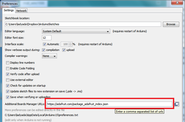
Open the Arduino IDE and go to File->Preferences and look for Additional Board Manager URLS. Add the following line to the manager:

https://adafruit.github.io/arduino-board-index/package_adafruit_index.json

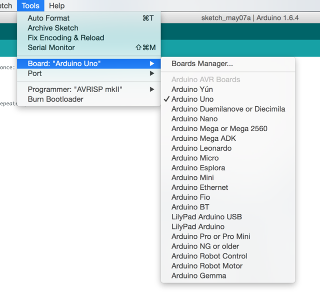
Now go to *Tools->Board->Boards Manager...*.

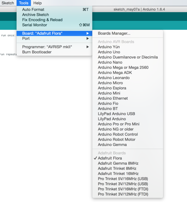
For Type choose Contributed and install Adafruit AVR Boards.

<video width="100%" controls> <source src="/images/2017-03-15-install.mp4" type="video/mp4"> Your browser does not support the video tag. </video>

Success looks like this:

More info

Step 5: Install the Adafruit nRF51 BLE Library

Acquire the Adafruit nRF51 BLE Library from here.

Rename the uncompressed folder Adafruit_BluefruitLE_nRF51 and ensure it contains Adafruit_BLE.cpp and Adafruit_BLE.h (as well as a bunch of other files)

Place the Adafruit_BluefruitLE_nRF51 library folder your arduino/libraries/ folder. This folder should have been created when you acquired the Arduino IDE, but you may also need to create it yourself.

Restart the IDE.

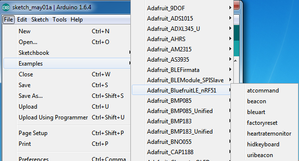
You'll know this worked if you see a number of examples in the menu File->Examples->Adafruit_Bluefruit_nRF51.

More info

Step 6: Get a BLE Dongle Working

Worried that my old phone wouldn't be able to work with BLE, I acquired this dongle.

Unfortunately, when I start it, I see this in dmesg | tail -n 20

[71112.636865] usb 1-1.1: new full-speed USB device number 10 using ehci-pci
[71112.749205] usb 1-1.1: New USB device found, idVendor=0a5c, idProduct=21e8
[71112.749210] usb 1-1.1: New USB device strings: Mfr=1, Product=2, SerialNumber=3
[71112.749213] usb 1-1.1: Product: BCM20702A0
[71112.749216] usb 1-1.1: Manufacturer: Broadcom Corp
[71112.749218] usb 1-1.1: SerialNumber: 5CF3707F3F1B
[71112.756203] Bluetooth: hci1: BCM: chip id 63
[71112.772214] Bluetooth: hci1: BCM20702A
[71112.773211] Bluetooth: hci1: BCM20702A1 (001.002.014) build 0000
[71112.773239] bluetooth hci1: Direct firmware load for brcm/BCM20702A1-0a5c-21e8.hcd failed with error -2
[71112.773243] Bluetooth: hci1: BCM: Patch brcm/BCM20702A1-0a5c-21e8.hcd not found

Let's fix that:

1. Open your favorite terminal

2. Acquire the driver file from me or from Amazon.

3. Run sudo mkdir /lib/firmware/brcm

4. Copy the firmware file to the /lib/firmware/brcm folder and rename the file to BCM20702A0-0a5c-21e8.hcd with, e.g.:

   sudo mv fw-0a5c_21e8.hcd /lib/firmware/brcm/BCM20702A0-0a5c-21e8.hcd

5. Now ensure all versions of this dongle work by running:

   sudo cp /lib/firmware/brcm/BCM20702A0-0a5c-21e8.hcd /lib/firmware/brcm/BCM20702A1-0a5c-21e8.hcd

TODO

AT+HWGETDIETEMP

sudo apt install gcc-avr avr-libc

Scientists are mirroring data from government sites, ensuring it does not vanish under the next U.S. administration.

As part of that effort, I've downloaded 11GB of NLCD data.

Now, how to make that available?

My plan is to spin up a node on DigitalOcean, which provides cheap cloud hosting, and make the data available via torrent.

Why Torrents?

They ensure the integrity of the file being downloaded, share bandwidth costs, facilitate speedy downloads, and enable users to easily participate in archiving data.

TODO

Instructions

Install the Transmission torrent client and daemon:

sudo apt install transmission-daemon transmission-cli

You'll now need a non-root user to run the daemon and handle the data. If you don't already have one, you can create one as follows:

sudo adduser --disabled-password transmission
sudo mkdir -p /home/transmission/Downloads
#Move the data files to the user's `Downloads` directory:
sudo mv TODO_FILES_HERE /home/transmission/Downloads
#Ensure permissions are set correctly
chown -R transmission /home/transmission/Downloads
chgrp -R transmission /home/transmission/Downloads

Create torrents for each file with transmission-create:

ls * | xargs -n 1 transmission-create

Move these torrents out of the directory:

mv *.torrent ~/

You can also create torrents of entire directories, ala:

:::bash transmission-create directory_name/

We now need to add trackers to the torrents. Below is a list of trackers which may work for you until dedicated Earth Science trackers can be set up. (TODO) The following command adds them to the torrent files:

echo "http://9.rarbg.com:2710/announce
http://announce.torrentsmd.com:6969/announce
http://bt.careland.com.cn:6969/announce
http://explodie.org:6969/announce
http://mgtracker.org:2710/announce
http://tracker.tfile.me/announce
http://tracker.torrenty.org:6969/announce
http://tracker.trackerfix.com/announce
http://www.mvgroup.org:2710/announce
udp://9.rarbg.com:2710/announce
udp://9.rarbg.me:2710/announce
udp://9.rarbg.to:2710/announce
udp://coppersurfer.tk:6969/announce
udp://exodus.desync.com:6969/announce
udp://glotorrents.pw:6969/announce
udp://open.demonii.com:1337/announce
udp://tracker.coppersurfer.tk:6969/announce
udp://tracker.glotorrents.com:6969/announce
udp://tracker.leechers-paradise.org:6969/announce
udp://tracker.openbittorrent.com:80/announce
udp://tracker.opentrackr.org:1337/announce
udp://tracker.publicbt.com:80/announce
udp://tracker4.piratux.com:6969/announce" | xargs -n 1 -I {} transmission-edit -a {} *.torrent

Start the daemon with transmission-daemon:

transmission-daemon -er -GSR -T

The -er flag enforces peer encryption. The -GSR flag seeds regardless of the ratio of upload to download, which is important since I hope to do quite a bit of seeding. -T says we don't require authentication.

(For debugging the above use the -f foreground flag. You can indicate an alternative downloads directory with -w DIRNAME.)

Add the torrents:

ls *.torrent | xargs -n 1 transmission-remote --add

If you check on the status of the daemon:

transmission-remote -l

It should have recognized that the torrents were already present in the Downloads directory and be ready to seed them, like so:

ID     Done       Have  ETA           Up    Down  Ratio  Status       Name
   1     0%       None  Unknown      0.0     0.0   None  Idle         NLCD_canopy_legend_2013.jpg
   2   100%   254.6 MB  Done         0.0     0.0    0.0  Idle         ak_nlcd_2011_landcover_1_15_15.zip
   3   100%   268.3 MB  Done         0.0     0.0    0.0  Idle         AK_nlcd_2011_USFS_tree_canopy_2011_edition_2016_02_08_analytical.zip
   4   100%   89.55 MB  Done         0.0     0.0    0.0  Idle         AK_nlcd_2011_USFS_tree_canopy_2011_edition_2016_02_08_cartographic.zip
   5   100%    1.21 MB  Done         0.0     0.0    0.0  Idle         ak_nlcd_2011_zone8_impervious_1_15_15.zip

If all of the files show Done as being 0%, then you may have the files located in the wrong place. Ensure they are in the directory indicated by

transmission-remote -si

The output of which includes this:

CONFIG
  Download directory: /home/rick/Downloads   <-Ensure your files are here

Alternatively, you may need to recreate and re-add one or all of the torrents as occasionally, for reasons unknown to me, this does not work the first time. Torrents can be removed with:

transmission-remote -t <ID#> -r

Magnet Links

Time was when you had to share torrent files in order for someone to get access to your torrent. Now, we have magnet links. They have have the same information, but without the clumsy files. To generate magnet links for your torrents, use the following:

ls *.torrent | xargs -n1 sh -c 'echo "\n$0"; transmission-show -m $0'

But You Wanted A Server

Here's an easy way to set up a file-sharing server:

sudo apt install nginx

Edit the configuration like so:

sudo pico /etc/nginx/nginx.conf

So that it includes the following indicated line:

http {

        ##
        # Basic Settings
        ##

        autoindex on;   #This is the import bit

Delete the default landing page:

rm -f /var/www/html/*

Move the torrent files, data, and other directories into:

mv *.torrent /var/www/html/

Ensure that they can be read by the webserver:

chmod -R a+r /var/www/html/*

And you're ready to roll.

I frequently load large numbers of layers into QGis. They all get normalized independently, which makes it difficult to compare them. So here's a chunk of Python code which normalizes them all together.

def GetAllLayersMinMax():
  minval = float('Inf')
  maxval = -float('Inf')
  for l in iface.legendInterface().layers():
    stats = l.dataProvider() \
                 .bandStatistics(
                    l.renderer().usesBands()[0], 
                    QgsRasterBandStats.All, 
                    l.extent(), 
                    0)
    minval = min(minval,stats.minimumValue)
    maxval = max(maxval,stats.maximumValue)
  return (minval,maxval)

def NormAllLayerColours(minval,maxval):
  for l in iface.legendInterface().layers():
    myType               = l.renderer().dataType(l.renderer().usesBands()[0])
    myEnhancement        = QgsContrastEnhancement(myType)
    contrast_enhancement = QgsContrastEnhancement.StretchToMinimumMaximum
    myEnhancement.setContrastEnhancementAlgorithm(contrast_enhancement,True)
    myEnhancement.setMinimumValue(minval)
    myEnhancement.setMaximumValue(maxval)
    l.renderer().setContrastEnhancement(myEnhancement)
    l.triggerRepaint()

#Use this
NormAllLayerColours(*GetAllLayersMinMax())

#Or this
NormAllLayerColours(1,1000)

Installing Lubuntu 16.04 was pretty easy, but, as regular Linux users know, there are usually a couple of sharks hiding that you have to dispatch before your system will work perfectly.

#Internet Stops Working

After running the system for a while the wireless internet will stop working.

Dutifully, I run:

sudo service network-manager restart

But this returns the message:

Failed to add /run/systemd/ask-password to directory watch: No space left on device

But I have lots of space available on the hard disk, in RAM, and via swap. What's going on?

As discussed here, it turns out that the Crashplan back-up service, which I have, is the most likely culprit. It uses many inotify watches and, eventually, eats them all up.

The immediate fix is to run:

sudo -i
echo 1048576 > /proc/sys/fs/inotify/max_user_watches
exit

To make more watches available.

The long-term fix is to edit the file /etc/sysctl.conf to include the line:

fs.inotify.max_user_watches=1048576

It's been a few days now and the problem hasn't returned since I did the above.

#Disppearing text in Thunderbird and Alt+Tab

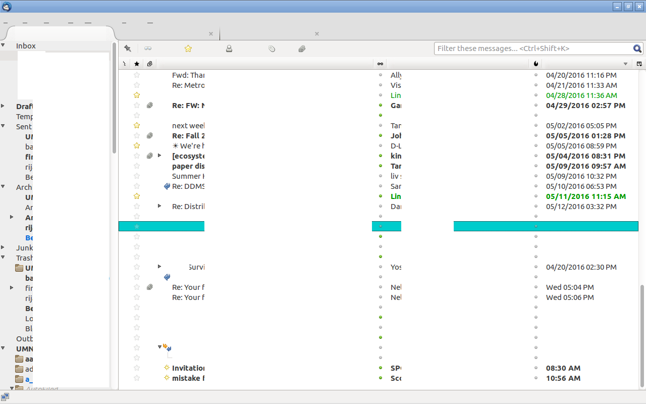
Whole message lines disappear in the Thunderbird mail client. The Alt+Tab switcher shows icons, but shows no text.

It looks like this (I've whited out most of the columns for privacy, but you can see the issue in terms of lines that have no text):

Closing Thunderbird and reopening resolves the problem until the next time the computer is put to sleep and wakes up again.

Running from the command line did not generate any useful debugging information.

Status: This somehow resolved itself, or I fixed it and don't remember how.

#Can't hover over an lxpanel menus

Status:

Running killall lxpanel and lxpanel & from the command line yield a panel which worked. Running meld on

I wanted to use my Tablet as a touchscreen monitor for my computer.

To do so, I installed Vino:

sudo apt-get install vino

Disabled the encryption (I'm on a secure intranet):

gsettings set org.gnome.Vino require-encryption false

And started the server:

/usr/lib/vino/vino-server &

On Android, I downloaded bVNC

And connected to port 5900.

Magic ensued.

A 1:1 size ratio between the tablet and the monitor would be helpful: it's difficult to get the mouse pointing in the right direction.

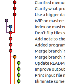
I have a Git repo I'm about to release because Science. Unfortunately, its history is a bit messy and I don't necessarily want people to know about the embarrassing mistakes and backtracks I made, or the kind of time I put into the code.

But I don't want to ditch that history either. What I want then is a way to separate the history of the master branch out into a private branch leaving the master on its own.

Let's do this!

#Rename master to old_master
git branch -m master old_master
#Find the most recent commit on old_master
git log
#Create, and switch to, a new master branch
git checkout --orphan master fb33e2286ffe90641f34c078a81a94e393dc30b8 
#Commit the new master
git commit -m "Public release"
#Push up the branch, overwriting history:
git push --set-upstream origin master --force

Now things are good to go.

This will embarrass me later, when I think of a better solution. But, sometimes, you need a fast and dirty answer.

I want a modulus operator Mod(a,b,m) such that:

• Mod(2,6,7)=-3
• Mod(6,2,7)=3

That is, the operator avoids the 4-hop path between 2 and 6 and, instead, circles around via a path of length 3. The answer preserves the path direction if you leave from a and go to b.

The following code calculates this. There's got to be a better way.

#include <iostream>
#include <cmath>

double absmin(double a, double b){
  if(std::abs(a)<std::abs(b))
    return a;
  else
    return b;
}

double ModDist(double src, double dest, double m){
  if(dest<src)
    return absmin(dest+m-src, dest-src);
  else
    return absmin(dest-src, dest-m-src);
}

int main(){
  std::cout<<ModDist(2,6,7)<<std::endl;
  std::cout<<ModDist(6,2,7)<<std::endl;
}

Get access to a compute node so that you have full memory and processing resources:

salloc -N 1 -t 120

Get Julia!

wget https://github.com/JuliaLang/julia/releases/download/v0.4.5/julia-0.4.5-full.tar.gz

Unpack and switch into the directory

tar xvzf julia-0.4.5-full.tar.gz
cd julia-0.4.5

Configure the Make.user file (which does not exist, yet) so that we take advantage of Intel's goodies:

USEICC = 1
USEIFC = 1
USE_INTEL_MKL = 1
USE_INTEL_MKL_FFT = 1
USE_INTEL_LIBM = 1

Figure out where ICC is hiding which icc

Load its compiler variables (e.g.):

source /opt/intel/composer_xe_2013_sp1.2.144/bin/compilervars.sh intel64

Make things (with many cores)!

make -j 24

Things stop working. Run make to get back to the error message.

Get this error:

Warning: git information unavailable; versioning information limited
Warning: git information unavailable; versioning information limited
  GEN      src/unix/uv-dtrace.o
gcc: error: unrecognized command line option ‘-static-intel’
"gcc /tmp/tmplsN9bM.c" failed
Usage /usr/bin/dtrace [--help] [-h | -G] [-C [-I<Path>]] -s File.d [-o <File>]
make[3]: *** [src/unix/uv-dtrace.o] Error 1
make[2]: *** [all] Error 2
make[1]: *** [libuv-efb40768b7c7bd9f173a7868f74b92b1c5a61a0e/.libs/libuv.la] Error 2
make: *** [julia-deps] Error 2

Fix it:

export CC=icc

Make things!

make -j 24

Things stop. Run make to figure out why.

Get this error:

Warning: git information unavailable; versioning information limited
    JULIA usr/lib/julia/inference0.ji
could not allocate pools
/bin/sh: line 1:  8512 Aborted                 /home/rbarnes1/temp/julia-0.4.5/usr/bin/julia -C native --output-ji /home/rbarnes1/temp/julia-0.4.5/usr/lib/julia/inference0.ji -f coreimg.jl
make[1]: *** [/home/rbarnes1/temp/julia-0.4.5/usr/lib/julia/inference0.ji] Error 134
make: *** [julia-inference] Error 2

Fix it:

pico src/gc.c

Find Line 165. It looks like this:

#define REGION_PG_COUNT 16*8*4096 // 8G because virtual memory is cheap

make it look like this:

#define REGION_PG_COUNT 8*4096 // 8G because virtual memory is cheap (becomes 512MB)

Make things!

make -j 24

Victory!

Create a symbolic link to julia-0.4.5/usr/bin/julia from wherever your bin directory is, or set up an appropriate alias.

More Info:

• Julia Issue 14807

I have a Lenovo Thinkpad X201 that I use for all things.

It has a blue button near the top that, currently, doesn't do anything:

I want this button to do something awesome.

How?

First, I need it's keycode:

sudo apt-get install xbindkeys
xbindkeys --defaults-guile > ~/.xbindkeysrc.scm
xbindkeys --key

Then I press The Key. This returns:

Press combination of keys or/and click under the window.
You can use one of the two lines after "NoCommand"
in $HOME/.xbindkeysrc to bind a key.
"NoCommand"
    m:0x0 + c:156
    XF86Launch1

Great, so I know it's keycode is 156 and, even better, it has a symbol XF86Launch1.

I've gotta clean up that config file:

rm ~/.xbindkeysrc.scm

Great. Now, I'll edit ~/.config/openbox/lubuntu-rc.xml to read:

<keyboard>
  ...
  <keybind key="XF86Launch1">
    <action name="Execute">
      <command>/home/my_user/bin/_blue_key_of_doom_</command>
    </action>
  </keybind>
  ...
</keyboard>

Running openbox --reconfigure reloads the keybindings. And, sure enough, the test script runs.

For now, I'll just make the script execute

xterm -fullscreen -e cmatrix

which will immediately plunge the screen into the Matrix.

You have some C/C++ code that you've used to build a package for R. Now you'd like to profile that code. How do you do it?

You can compile your package for use with, e.g.,

R CMD INSTALL --no-multiarch --clean .

But, you'll notice that R is quite insistent about including the -g -O2 compiler flags, which can complicate debugging.

Therefore, create the file $HOME/.R/Makevars

And, assuming your my_package/src/Makevars file contains

CXX_STD = CXX11

Use the following line to override R's optimization flags:

CXX1XFLAGS += -Og

Note that -Og is an optimization level that is ... optimized for debugging purposes. Different flag lines (such as CXX1XFLAGS) work for various versions of the standard.

You can then install oprofile using

sudo apt-get install oprofile

And build a test script containing code that will evoke the functions/methods you wish to profile. Run this script using:

operf R -f tests.R

The summary results can be viewed with:

opreport

And the timing of your library with:

opreport -l ~/R/x86_64-pc-linux-gnu-library/3.2/my_package/libs/my_package.so

Source files annotated with the samples per line can be generated with:

opannotate --source ~/R/x86_64-pc-linux-gnu-library/3.2/my_package/libs/my_package.so

The output appears as follows:

samples  %        image name               symbol name
2013892  66.7818  my_package.so            MyClass::hot_method(std::vector<double> const&)
831090   27.5594  my_package.so            MyClass::another_method(unsigned long)
69978     2.3205  my_package.so            void DoStuff(int,int,double)
56868     1.8858  my_package.so            int AdjustThings(unsigned long, unsigned long)
8845      0.2933  my_package.so            MyClass::cheerios(int)

Oprofile works by checking in periodically to see where your code is at. The first line is the number of these samples that occurred in each function (listed at right), while the second column is the percent of the total samples this represents.

The foregoing indicates that MyClass::hot_method() is probably where optimization efforts should be focused.

The annotated output appears as follows:

:        nearest_neighbors.push_back(which_lib[0]);
118511  3.9299 :        for(auto curr_lib: which_lib)
               :        {
  3219  0.1067 :            curr_distance = dist[curr_lib];
1398851 46.3867 :            if(curr_distance <= dist[nearest_neighbors.back()])
               :            {
               :                i = nearest_neighbors.size();
123725  4.1028 :                while((i > 0) && (curr_distance < dist[nearest_neighbors[i-1]]))
               :                {
               :                    i--;
               :                }
               :                nearest_neighbors.insert(nearest_neighbors.begin()+i, curr_lib);

Here the first column is again the number of samples and the second column is again the percentage of the total samples this represents. This gives a pretty good idea of where the bottleneck is.

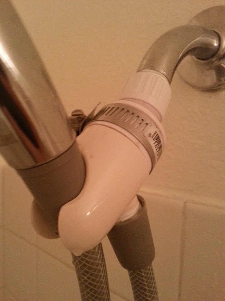
My bathroom sinks burbled and sprayed. It's bothered me ever since I moved in, but I've been busy fixing other things (carpets vacuum shampooed? yup). Inspired by Jeroen De Wilde's roaster, I decided the time had come to tackle this. Little did I know that it would lead me down a rabbit hole of alternatives analysis, proprietary design, and vendor lock-in. The story unfolds below.

This sink burbles and sprays. It gets water everywhere, lacks aesthetics, wastes water, and seems unhygienic (I don't know why I feel this way about the latter bit). BUT IT IS TOTALLY FIXABLE!

A little genlte work with the vise-grip wrench to the aerator off and showed that, indeed, the sink had good flow. That isolated the issue.

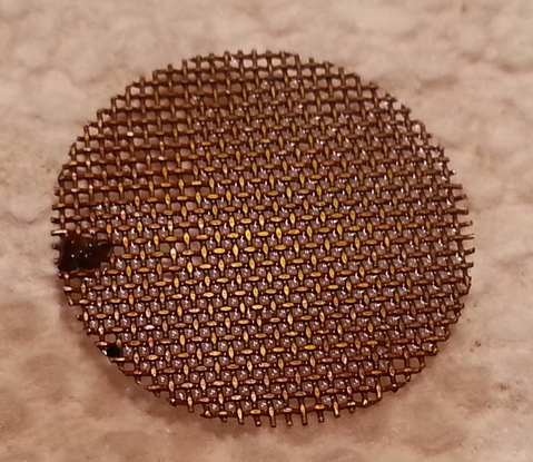
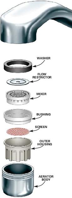
Speaking of the aerator&hellip; here are the parts I got out of it. A double-stacked screen, a basket for the screen, a top for the basket, and a rubber O-ring. The second sink was missing the O-ring&hellip; someone opened these sinks before and didn't appropriately reassemble them.

Sadly not photographed were the little rocks and hard gunk on the screens. If this aerator weren't missing parts (see the next photo), cleaning that gunk off probably would have fixed the issue and I'd have been done. A picture of some new gunk I found is shown below: the old stuff was harder and larger.

So, my old aerator was missing parts: the restrictor and mixer were just&hellip; gone. It's easy to imagine losing an O-ring down the drain accidentally, but hard to imagine how the last fixer-upper lost these pieces.

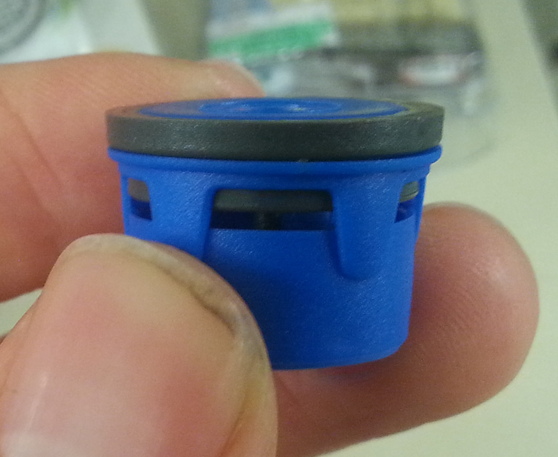
Replacement Candidate #1: Plumb Park's Auto-Cleaning Aerator. The Ace Hardware person recommended this because its metal casing would "fit". Turns out: lots of metal casings fit and the hardware store has a handy thing you can screw your old aerator into so you get the sizing right.

This aerator was a clear reject. The idea (see next picture) is to do a first flush to get debris off the top screen, then close the gap with the washer to initiate aeration.

The problem? That's a big hole on the top and the screen at the bottom is fine mesh: this thing's going to get loaded with junk, I won't be able to clean it, and I'll have to buy a new one within (possibly) weeks. That's a no go.

An example of epic over-engineering failing. This design would have a certain charm&hellip; if the holes at the bottom were big enough to let gunk out. But they're not, so this aerator, far from being self-cleaning is more like self-filthing.

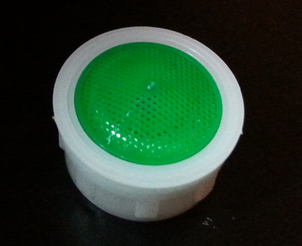
Replacement Candidate #2: The "Cyclone" Aerator. Barely visible on the top of this aerator (sorry for the bad angle) is a big hole.

Naturally, the bottom is a fine, inaccessible mesh. This is another aerator asking to get clogged.

And here it is: fine mesh on the top to keep that big crud from getting in. Fine mesh on the bottom to help break up the flow. It's not self-cleaning, but I know how to use a wrench, so who cares?

But this is where things took a turn for the sad. Turns out all of the aerators I just showed you are sized to within millimetres of each other. But different millimetres, such that none of them are interchangeable in the metal casings of the other vendors. So, instead of picking up two $3 aerators, I need two $7 aerator+casings&hellip; or I can buy six of them in bulk for $16.

But the flow's fixed, so that's okay.

An ARC/INFO ASCII GRID file is a format for storing (among other thing) digital elevation models and looks like the following:

ncols         4
nrows         6
xllcorner     0.0
yllcorner     0.0
cellsize      50.0
NODATA_value  -9999
-9999 -9999 5 2
-9999 20 100 36
3 8 35 10
32 42 50 6
88 75 27 9
13 5 1 -9999

The fields define the number of columns and rows, the latitude and longitude (or whatever coordinate system is being used), the dimensions of the grid cells (in the same coordinate system), and a value which indicates that no data is available for a particular cell. Following this, there is a rectangular array of ASCII-encoded numbers representing the digital elevation model.

The following function prints a 2D NumPy array in this format:

def writeArrayToArcGrid(arr,filename,xll,yll,cellsize,no_data_val):
  arr                = np.copy(arr)
  arr[np.isnan(arr)] = no_data_val
  headerstring       = bytes('NCOLS %d\nNROWS %d\nXLLCENTER %f\nYLLCENTER %f\nCELLSIZE %f\nNODATA_value %f\n' %
    (arr.shape[1], arr.shape[0], xll, yll, 1, no_data_val), 'UTF-8')

  with open(filename,'wb') as fout:
    fout.write(headerstring)
    np.savetxt(fout,arr,'%5.2f')

Thinking about the connections between environment and health, I extracted my data from Fitbit's grubby, proprietary paws for some analysis-lite.

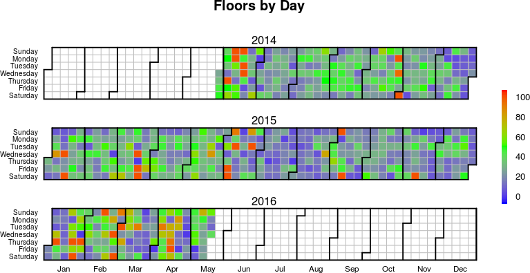
The following chart shows flights of stairs climbed per day (truncated to 100 floors per day to prevent instances of mountain climbing from skewing the figure).

During 2014 through June 2015 I lived on the fourth floor of a building whose kitchen was on the ground floor, and worked on the fifth floor of another building. This ensured a minimum of 18 flights of stairs per day and, often, much more.

From July 2015 through December 2015, I lived on a second floor and worked on a third floor. This mandated only 6 flights of stairs per day. And, indeed, this period shows far fewer stairs climbed on average.

In late January of 2016, I moved half-way up a rather large hill and continued to work on a third floor: stair climbing counts immediately rose.

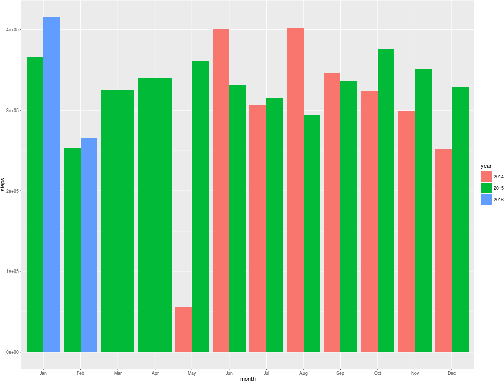
The following chart shows total steps taken per month. I was in a cold place for most of 2014 (red), spent the summer of 2015 (green) travelling, and was in warmer places from August 2015 (green and blue, sorry colour-blind folks) onwards. The gap in step counts, especially evident October through January, can therefore probably be attributed to a warmer climate being more conducive to moving about.

[This post was updated on 02016-06-06 to reflect the complete data from Spring 2016.]

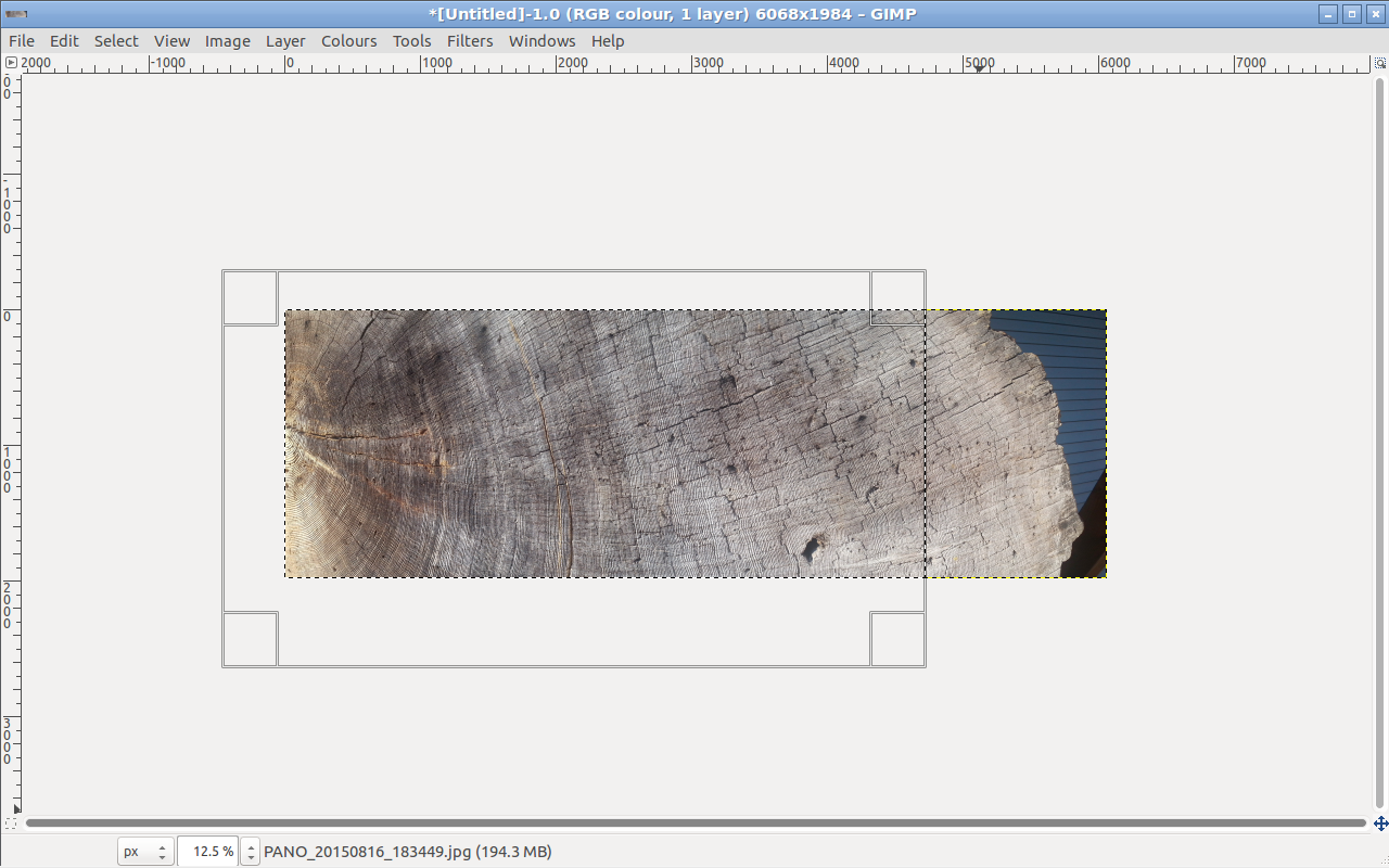
I saw this cross-section of a tree in La Connor, WA. Unusually, perhaps, for such a large tree, there was no nearby sign telling how old it was. Curious, I thought of a couple of ways to quickly get data so I could figure it out later.

#Image Analysis

The Google Camera app has a Panorama setting, which allowed me to get the above photo. So now it's possible for me to count the rings one by one, but that's boring, and isn't an easily repeatable solution.

If we look closer, though, each ring of the tree forms a convenient little ridge. At this lighting angle, they leave little shadows. We can work with this.

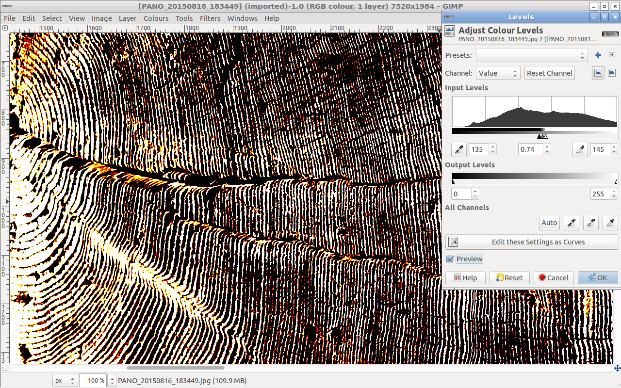
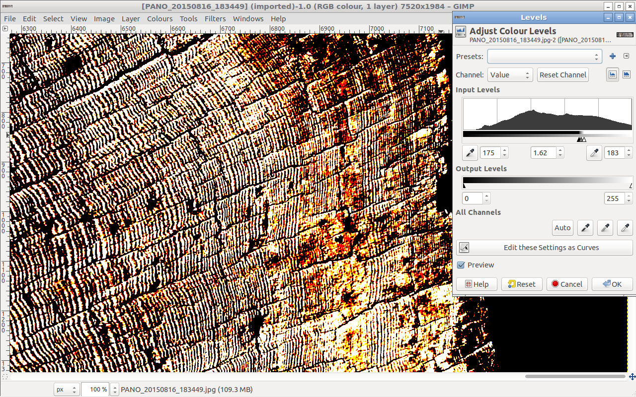
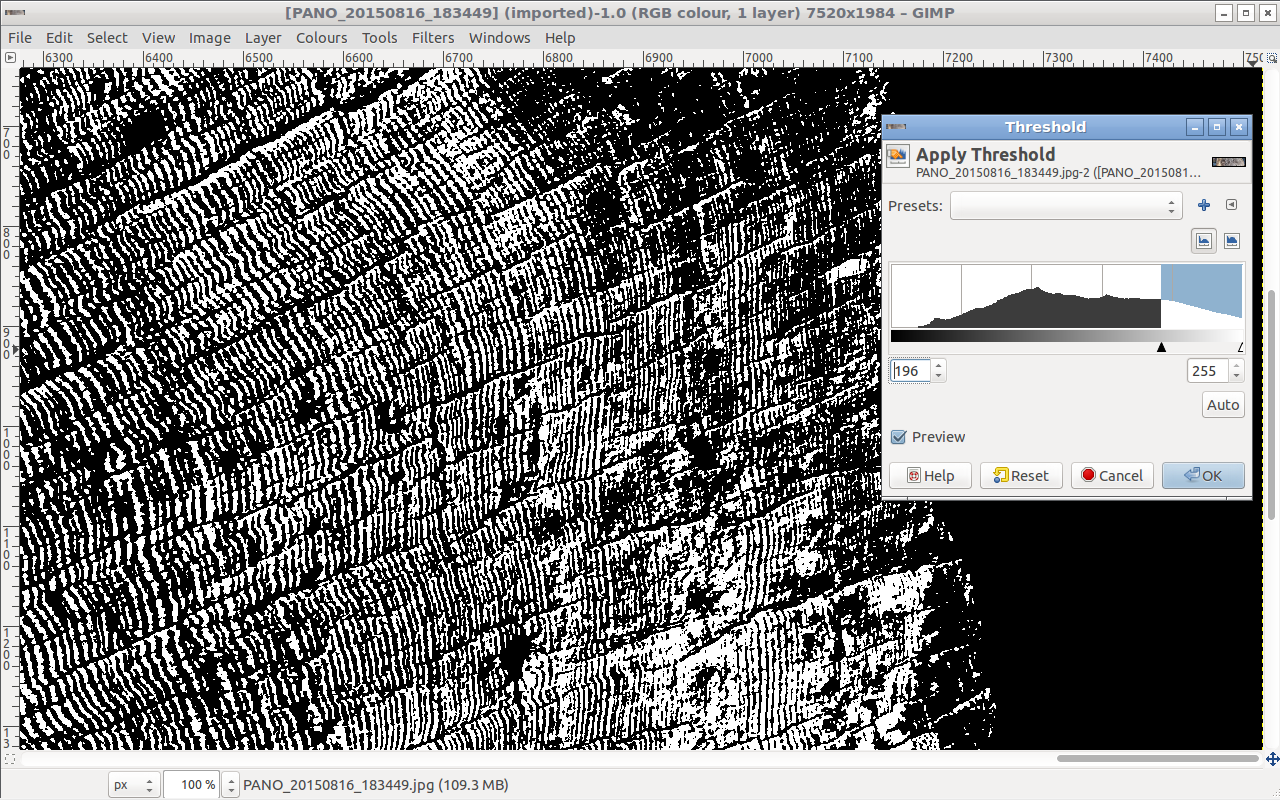
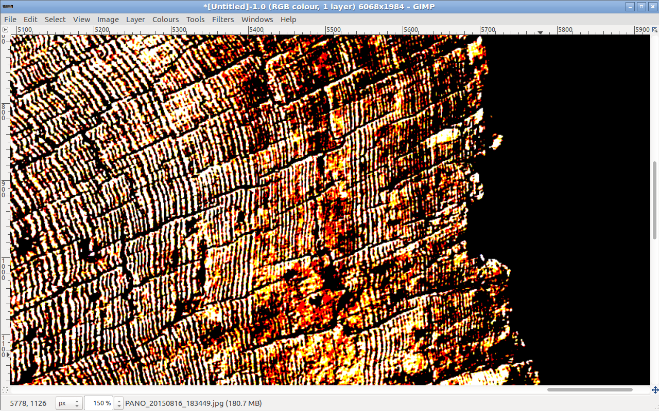
So I pulled out GIMP, cropped the image so that it included only the right-hand side of the tree, and fiddled with the Levels and Threshold settings to come up with a couple of black-and-white images.

Since the illumination and relative angle of the ridges changes across the diameter of the trunk, I also tried processing it in chunks.

The end result is a black and white image: a binary matrix.

Here's a zoom in on part of the above image.

I can now load this into R and find the number of tree rings like so:

library(png)
img<-readPNG("bw_tree_rings.png))

#Get only one of the dimensions. It doesn't matter
#which one since this is a binary matrix so the RGB
#channels are all equal
img<-img[,,1]

#Check that a cross-section of the image is as expected
length(img[1,])

#If it wasn't, we could transpose. But it was, so we're good
#img<-t(img)

#Display the image
image(img, asp=1,axes=FALSE,useRaster=TRUE)

#Each row of the matrix is something like "0,0,0,1,1,1,0,1,1".
#Differentiating this gives "0,0,0,1,0,-1,0,1,0". Each value
#of "1" corresponds to a new ridge. Summing all the "1" values
#gives the number of tree rings. I do this for each row like so.
a<-apply(img, 1, function(x) sum(diff(x)>0))

#Print out a plot of tree rings versus image row
png('/z/tree-plot.png', width=6, height=6, units="in", res=300)
plot(a,xlab="Row", ylab="Tree Rings")
dev.off()

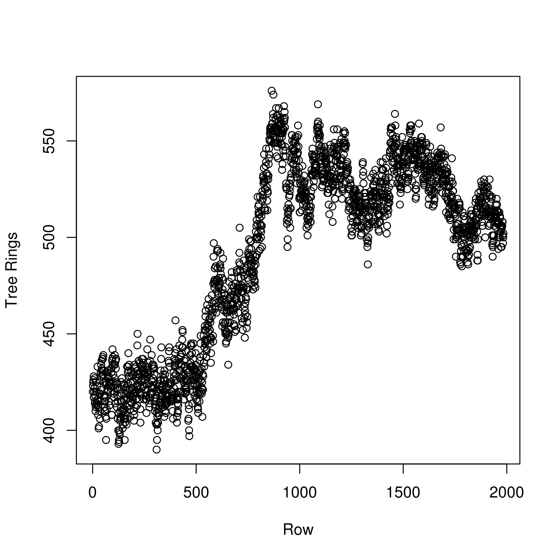
Which gives the following plot:

Naturally, since not every row is a diamater, most of the above plot is rubish. But, looking at the original image, we see that the center of the tree is situated just off-center (vertically) of the image. Since the image is 2000 pixels tall, we are looking for a patch of data just to one side of the mid-point; here, that corresponds to the data points around row 950 or so.

This establishes the age of the tree as approximately 550&ndash;600 years old, though the latter is true only if you believe the highest data points.

#Using the accelerometer

Since each tree ring formed a little ridge, another way to count the rings was to run AndroSensor at a high-frequency to collect my phone's accelerometer data. Holding the phone tightly in my hand to reduce damping, I ran my finger nail across a diameter of the tree. Each tree ring ridge resulted in a little bump, which the accelerometer would record.

The resulting data looks like this.

|ACCELEROMETER X (m/s²)|ACCELEROMETER Y (m/s²)|ACCELEROMETER Z (m/s²)|Time since start in ms |YYYY-MO-DD HH-MI-SS_SSS|
|-1.152|6.942|6.2474|14|2015-08-16 18:24:28:322|
|-1.152|6.942|6.2474|19|2015-08-16 18:24:28:327|
|-1.152|6.942|6.2474|36|2015-08-16 18:24:28:344|
|-1.152|6.942|6.2474|49|2015-08-16 18:24:28:357|
|-0.9712|6.9156|6.451|58|2015-08-16 18:24:28:366|
|-0.9712|6.9156|6.451|64|2015-08-16 18:24:28:372|
|-0.9712|6.9156|6.451|67|2015-08-16 18:24:28:375|
|-0.9712|6.9156|6.451|75|2015-08-16 18:24:28:383|
|-0.8442|7.1443|6.7132|78|2015-08-16 18:24:28:386|
|-0.8442|7.1443|6.7132|80|2015-08-16 18:24:28:388|

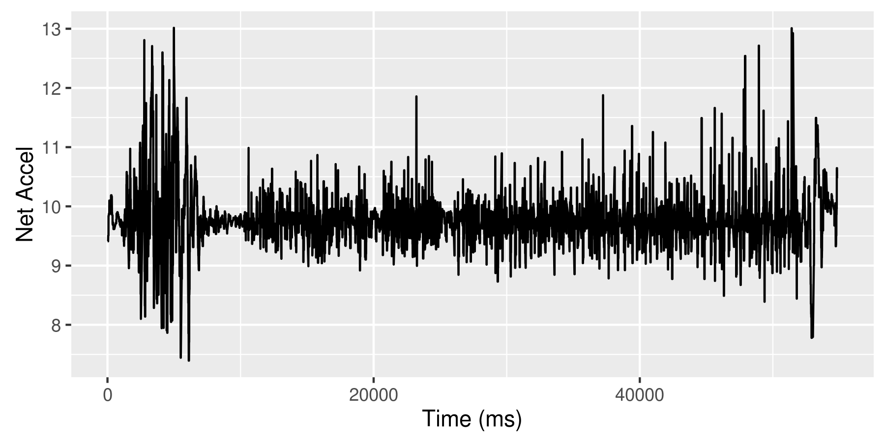
Plotting the vector norm of the acceleration, the entire data set looks like this:

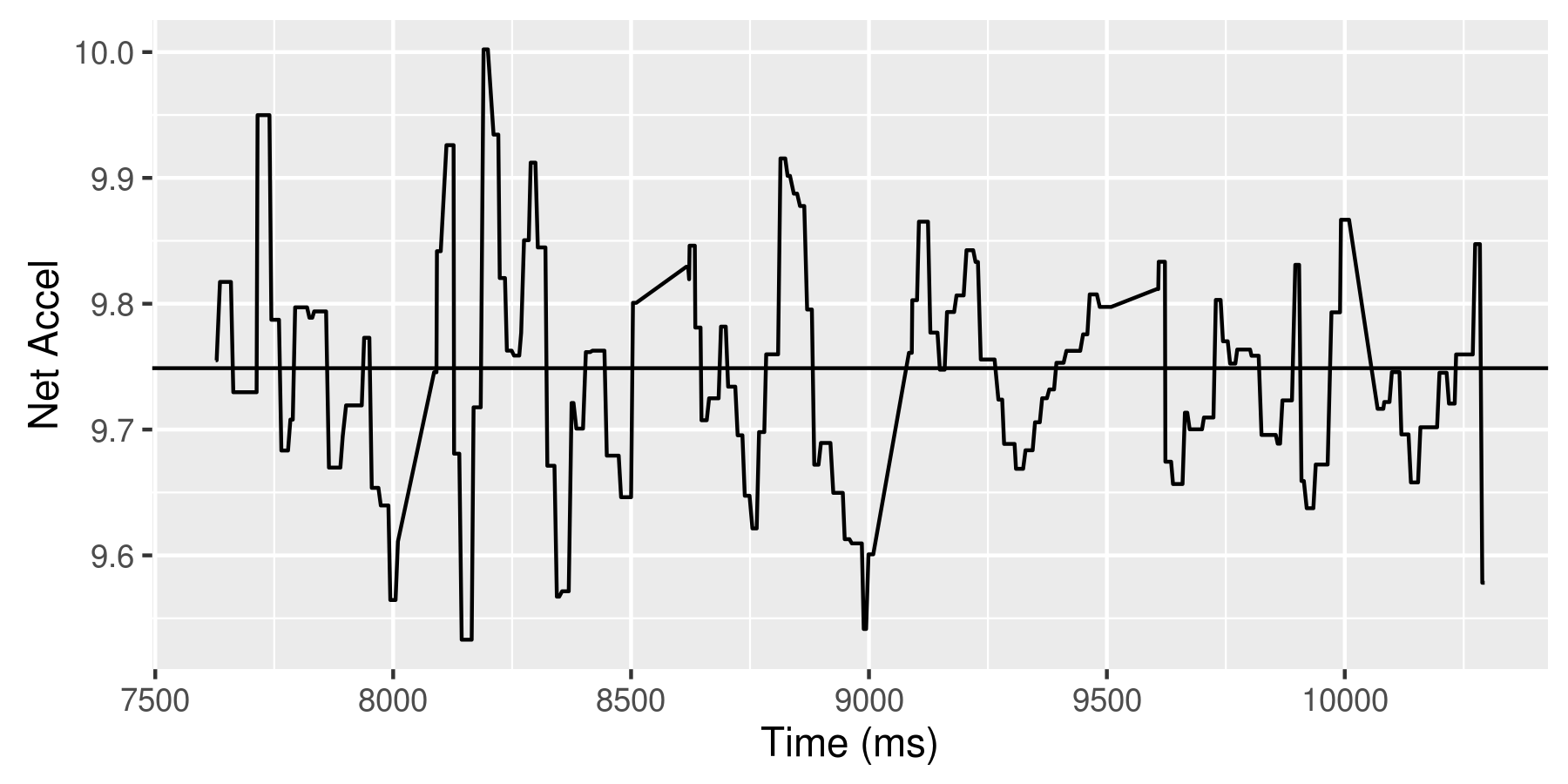
The first bit is me testing trying out the method. Then there's a quiet bit where I simply hold the phone with my finger resting on the tree. This gives me some calibration data so I can get a sense of how the accelerometer's background noise. Next, I begin running my fingernail across the tree trunk. There are occasional pauses as I relocate my body.

The calibration data looks a bit like this.

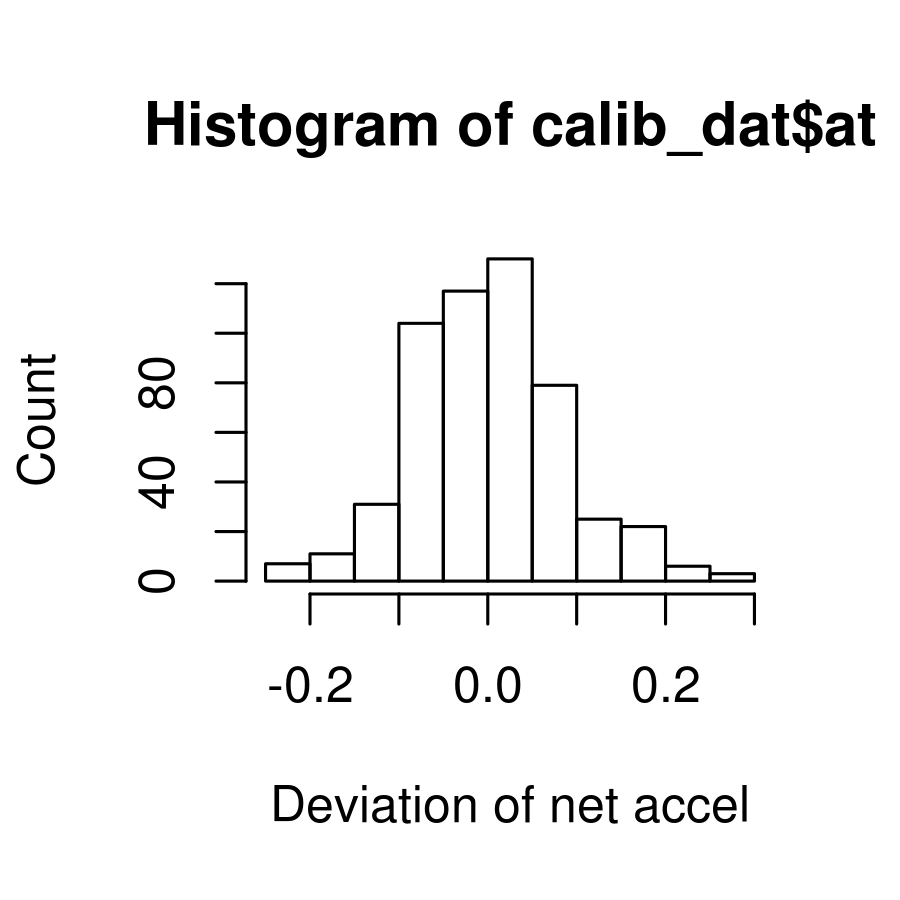
The distribution of the calibration data about its mean is

From the foregoing, it seems reasonable to classify every data point within 0.1 of the mean as being noise. Therefore, I manipulate the data by tossing out the negative side of the waveform (since every acceleration is followed by a deacceleration) and then removing all data beneath this noise threshold. I can then approximate the age by differentiating the signal and counting rises.

This gives 502 tree rings.

A hand count (I had to know!) gives 672 rings, so it seems that both of the methods I used were a bit losy.

The code for that is as follows:

library(ggplot2)

file='Sensor_record_20150816_182523_AndroSensor.csv'
dat<-read.csv(file, sep=';')
dat<-data.frame(dat)
colnames(dat)<-c('ax','ay','az','ms','date')
dat$at<-sqrt(dat$ax**2+dat$ay**2+dat$az**2)
head(dat)

#Show all the data
png('/z/tree-sound.png', width=6, height=3, units="in", res=300)
ggplot(dat)+geom_line(aes(x=ms,y=at))+ylab("Net Accel")+xlab("Time (ms)")
dev.off()

#Find the calibration period start and end times with
#plotting and some trial and error
calibration_period<-(7625<dat$ms & dat$ms<10295)
calib_dat<-dat[calibration_period,]
#plot(calib_dat$ms,calib_dat$at)

#Get the mean of the calibration data
datmean<-mean(calib_dat$at)

#Plot calibration period
png('/z/tree-calib.png', width=6, height=3, units="in", res=300)
ggplot(calib_dat)+
  geom_line(aes(x=ms,y=at))+
  xlab("Time (ms)")+
  ylab("Net Accel")+
  geom_hline(yintercept=datmean)
dev.off()

#Shift the data so it is centered about the mean
calib_dat$at<-calib_dat$at-datmean

#Plot a histogram of the shifted calibration data
png('/z/tree-hist.png', width=3,height=3,units="in",res=300)
hist(calib_dat$at, xlab="Deviation of net accel", ylab="Count", title="")
dev.off()

#Note that most of the noise falls within +/-0.1 of the mean,
#and nearly all falls within +/-0.2

#Shift all of the data and take a peek
dat_period<-(10790<dat$ms & dat$ms<51489)
dat_dat<-dat[dat_period,]
dat_dat$at<-dat_dat$at-datmean

ggplot(dat_dat,aes(x=ms,y=at))+geom_line()+ylim(-1,1)#+xlim(25000,30000)

#Keep only the positive side of the waveform
dat_dat[dat_dat$at<0,]$at<-0

ggplot(dat_dat,aes(x=ms,y=at))+geom_line()+ylim(-1,1)+xlim(25000,30000)

#Remove the noise
dat_dat[dat_dat$at<0.1,]$at<-0

ggplot(dat_dat,aes(x=ms,y=at))+geom_line()+ylim(-1,1)+xlim(20000,30000)

#Count all the rises. This is an approximation of the age.
sum(diff(dat_dat$at)>0)

Voxels are like 3d pixels and useful for various visualization tasks. I had some neuron-voxel data I wanted to plot. I also wanted this plot to be interactive such that I could freely rotate and zoom it to get a better sense of what was going on. The following MWE achieves this:

library(rgl)

#Generate a random set of voxel coordinates
data<-expand.grid(1:4,1:4,1:4)
data<-data[sample(nrow(data),20,replace=FALSE),]

#Generate random values
data$v<-runif(20)

#Give everything pretty names
colnames(data)<-c('x','y','z','v')

#Generate a colour gradient
cols<-heat.colors(100)

#We now have data of the form x,y,z,value

#Clear the display in case there's something else on it
rgl.clear()

#Set background colour
bg3d('white')

for(j in 1:nrow(data)){                      #For each voxel
  #Values are in range [0,1]. Multiply be len(cols) to get colour of cube
  col<-ceiling(length(cols)*data$v[j])
  #Createa a voxel
  cubit = cube3d(color=col, alpha=0.3)
  #cubit$vb is a 4 by n matrix of vertices in homogeneous coordinates. Each column is a point.
  #Cube is originally 2x2x2. We shrink it to a 1x1x1 cube in the positive octant.
  cubit$vb[cubit$vb == -1] = 0
  cubit$vb[1,]      = cubit$vb[1,]+data$x[j] #Add x to first row
  cubit$vb[2,]      = cubit$vb[2,]+data$y[j] #Add y to second row
  cubit$vb[3,]      = cubit$vb[3,]+data$z[j] #Add z to third row
  shade3d(cubit,add = TRUE,alpha=0.5)
  wire3d (cubit,add = TRUE,color=col)
}

#Capture the current camera angle
pp1<-par3d(no.readonly=TRUE)

#Go to a captured camera angle
par3d(pp1)

#Save the image to a file
snapshot3d("image3d.png")

Trying to install the R 3d-viz package rgl on my machine gives the error:

configure: error: missing required header GL/gl.h

To fix this:

sudo apt-get install mesa-common-dev

A new error appears:

configure: error: missing required header GL/glu.h

To fix:

sudo apt-get install libglu1-mesa-dev

Success!

How do you find the first number less than or equal to a needle in an STL container? The following code does this and provides tests to ensure things are working as expected. Although the code is written for a vector, it could be adapted to any container providing a ForwardIterator.

#include <algorithm>
#include <vector>
#include <iostream>

//Find the largest number less than or equal to a needle number
double FindLargestLessThanEqualNeedle(const std::vector<double> &v, double needle){
  auto up = std::upper_bound(v.begin(), v.end(), needle);
  if(up==v.begin())
    return v.front();
  else if(up==v.end())
    return v.back();
  else
    return *(up-1);
}

//Find the index of the largest number less than or equal to a needle number
size_t FindLargestLessThanEqualNeedleIdx(const std::vector<double> &v, double needle){
  auto up = std::upper_bound(v.begin(), v.end(), needle);
  if(up==v.begin())
    return 0;
  else if(up==v.end())
    return v.size()-1;
  else
    return up-v.begin()-1;
}

int main(){
  std::vector<double> v={{0,1,4,8,10,15,20}};
  std::cout<<FindLargestLessThanEqualNeedle(v,-1)<<std::endl;
  std::cout<<FindLargestLessThanEqualNeedle(v,25)<<std::endl;
  std::cout<<FindLargestLessThanEqualNeedle(v,8)<<std::endl;
  std::cout<<FindLargestLessThanEqualNeedle(v,9)<<std::endl;
  std::cout<<FindLargestLessThanEqualNeedle(v,10)<<std::endl;

  std::cout<<FindLargestLessThanEqualNeedleIdx(v,-1)<<std::endl;
  std::cout<<FindLargestLessThanEqualNeedleIdx(v,25)<<std::endl;
  std::cout<<FindLargestLessThanEqualNeedleIdx(v,8)<<std::endl;
  std::cout<<FindLargestLessThanEqualNeedleIdx(v,9)<<std::endl;
  std::cout<<FindLargestLessThanEqualNeedleIdx(v,10)<<std::endl;
}

How do you count bits?

Peter Wegner published a technique in the Communications of the ACM, Vol. 3 No. 5, Page 322 on May 1960 for doing so. The article is available here and has the doi 10.1145/367236.367286.

//Counts the number of bits that are "on"
//This is a method developed by Peter Wegner (doi: 10.1145/367236.367286)
template<class T>
T countbits(T a){
  unsigned int c; // c accumulates the total bits set in combined
  for (c = 0; a; ++c)
    a &= a - 1;   // clear the least significant bit set
  return c;
}

The following set similarity functions are written in C++ for easy integration with R using the sourceCpp command.

The first function computes the Jaccard index assuming inputs are unique, sorted integers where each integer denotes an element of a set. L1 and L2 are both sets.

/**
 * The Jaccard Similarity Coefficient or Jaccard Index is used to compare the
 * similarity/diversity of sample sets. It is defined as the size of the
 * intersection of the sets divided by the size of the union of the sets.
 *
 * INPUTS:
 *    L1: A list of unique, sorted integers denoting set elements.
 *    L2: A list of unique, sorted integers denoting set elements.
 *
 * RETURNS:
 *    Size(Intersection(L1,L2))/Size(Union(L1,L2))
 *
 * SIDE-EFFECTS:
 *    None: this is the 21st-century.
 *
 * COMPLEXITY:
 *    Time:  O(N1+N2)
 *    Space: O(1)
 */
// [[Rcpp::export]]
NumericVector JaccardSimilarity(const NumericVector L1, const NumericVector L2){
  int n1                = L1.size();   //Number of elmeents in set 1
  int n2                = L2.size();   //Number of elmeents in set 2
  int i1                = 0;           //Current element of interest in set 1
  int i2                = 0;           //Current element of interest in set 2
  int size_intersection = 0;           //Result: to be incremented in algorithm
  int size_union        = 0;           //Result: to be incremented in algorithm

  while(true){
    if(i1==n1){
      size_union += n2-i2;
      break;
    } else if (i2==n2){
      size_union += n1-i1;
      break;
    }

    if(L1[i1]==L2[i2]){        //Element is in both sets.
      i1++;                    //Therefore, we discard both the current element
      i2++;                    //from both sets and mark the current element as 
      size_union++;            //being part of both the union and the
      size_intersection++;     //intersection

    } else if(L1[i1]<L2[i2]){  //Element is only in the first set.
      i1++;                    //Throw it out
      size_union++;            //and mark it as a member of only the union

    } else if(L1[i1]>L2[i2]){  //Element is only in the second set.
      i2++;                    //Throw it out
      size_union++;            //and mark it as a member of only the union
    }
  }

  return NumericVector::create((double)size_intersection/(double)size_union);
}

The second function computes the Jaccard index assuming only that L1 and L2 are both sets whose integers indicate set members.

/**
 * The Jaccard Similarity Coefficient or Jaccard Index is used to compare the
 * similarity/diversity of sample sets. It is defined as the size of the
 * intersection of the sets divided by the size of the union of the sets.
 *
 * INPUTS:
 *    L1: A list of integers denoting set elements.
 *    L2: A list of integers denoting set elements.
 *
 * RETURNS:
 *    Size(Intersection(L1,L2))/Size(Union(L1,L2))
 *
 * SIDE-EFFECTS:
 *    None: this is the 21st-century.
 *
 * COMPLEXITY:
 *    Time:  O(N1+N2)
 *    Space: O(N1+N2) worst-case
 */
#include <unordered_map>
// [[Rcpp::export]]
NumericVector JaccardSimilarityUnsorted(const NumericVector L1, const NumericVector L2){
  int n1                = L1.size();   //Number of elmeents in set 1
  int n2                = L2.size();   //Number of elmeents in set 2
  int size_intersection = 0;           //Result: to be incremented in algorithm
  int size_union        = 0;           //Result: to be incremented in algorithm

  std::unordered_map<int, unsigned char> seen;

  for(int i1=0;i1<n1;i1++){            //Loop through all elements in Set 1
    if(!seen.count(L1[i1])){           //If we haven't seen the element before
      seen[L1[i1]] = 1;                //Mark it as having been seen in Set 1
      size_union++;                    //And as being part of the union
    }                
  }

  for(int i2=0;i2<n2;i2++){            //Loop through all elements in Set 2
    if(!seen.count(L2[i2])){           //If we have not seen the element before
      size_union++;                    //then it is part of the union.
      seen[L2[i2]] = 2;                //Mark it as being done.

    } else if(seen[L2[i2]]==1){        //Elsewise, we've seen the element in the
      size_intersection++;             //Set 1, it is part of the intersection
                                       //But not the union, because that would
                                       //be double counting.
      seen[L2[i2]] = 2;                //Mark it as being done.
    }
  }

  return NumericVector::create((double)size_intersection/(double)size_union);
}

This function, due to Jamie Murdoch, quickly computes the Fowlkes-Mallows index of a cluster assignment.

/**
 * Third iteration of the Fowlkes and Mallows similarity in C++.
 * For each cluster i, track the number of elements in that cluster.
 * For each pair of clusters (x, y), track the number of elements assigned to x
 *   in L1 and to y in L2. This is the "overlap" between x and y.
 * <C1, C1> is the sum of squares of cluster sizes. To see this, note that
 *   for all pairs of elements i, j in cluster x, c_{ij} = 1. For all pairs
 *   of elements in different clusters, c_{ij} = 0. Then, for each cluster x,
 *   the number of elements with value 1 in C_{ij} is |x|^2, the square of the
 *   cluster size. 
 * Another way to see this is that C_{ij} is an adjacency matrix for a graph, in
 *   which the clusters represent separate cliques. We want to count the number
 *   of edges for each clique, counting self-edges once and undirected edges
 *   between elements twice.
 * <C1, C2> is the sum of squares of overlap sizes. To see this, consider the
 *   overlap O_{xy} between clusters x and y. This is the number of elements that 
 *   belong to x in L1 and to y in L2. For any pair (i,j) of these elements,
 *   C_{ij} = 1 in both C1 and C2. This ordered pair contributes 1 to <C1, C2>.
 *   We sum these contributions across all pairs in the overlap (of which there
 *   are |O_{xy}|^2) and all overlaps.
 *
 * INPUTS:
 *    L1: Each item of the list is a point. The number stored at the element
 *        is the cluster the point is assigned to.
 *    L2: The same as L1. Must be the same length as L1.
 *
 * RETURNS:
 *    The Fowlkes and Mallows index
 *
 * SIDE-EFFECTS:
 *    None
 *
 * COMPLEXITY:
 *    Time:  O(K^2+n), where K = number of clusters
 *    Space: O(K^2)
 *
 * SOURCES:
 *    Asa Ben-Hur, Andre Elisseeff, and Isabelle Guyon (2001) A stability based
 *    method for discovering structure in clustered data. Biocomputing 2002: pp.
 *    6-17. 
 */
// [[Rcpp::export]]
NumericVector FowlkesMallows(const NumericVector L1, const NumericVector L2){
  int n = L1.size();
  int K = max(L1);

  ind overlaps[K][K];
  ind cluster_sizes1[K], cluster_sizes2[K];

  for(int i = 0; i < K; i++){
    cluster_sizes1[i] = 0;
    cluster_sizes2[i] = 0;
    for(int j = 0; j < K; j++)
      overlaps[i][j] = 0;
  }

  //O(n) time. O(K^2) space. Determine the size of each cluster as well as the
  //size of the overlaps between the clusters.
  for(int i = 0; i < n; i++){
    cluster_sizes1[(int)L1[i] - 1]++; // -1's account for zero-based indexing
    cluster_sizes2[(int)L2[i] - 1]++;
    overlaps[(int)L1[i] - 1][(int)L2[i] - 1]++;
  }

  // O(K^2) time. O(1) space. Square the overlap values.
  int C1dotC2 = 0;
  for(int j = 0; j < K; j++){
    for(int k = 0; k < K; k++){
      C1dotC2 += pow(overlaps[j][k], 2);
    }
  }

  // O(K) time. O(1) space. Square the cluster sizes
  int C1dotC1 = 0, C2dotC2 = 0;
  for(int i = 0; i < K; i++){
    C1dotC1 += pow(cluster_sizes1[i], 2);
    C2dotC2 += pow(cluster_sizes2[i], 2);
  }

  return NumericVector::create((double)C1dotC2 / (sqrt(C1dotC1) * sqrt(C2dotC2)));
}

We can modify the above to quickly compute the cluster assignment similarity using the Jaccard index, as suggested by Ben-Hur, Elisseeff, and Guyon (2002).

/**
 * The Jaccard Similarity Coefficient or Jaccard Index is used to compare the
 * similarity/diversity of sample sets. It is defined as the size of the
 * intersection of the sets divided by the size of the union of the sets. Here,
 * it is used to determine how similar to clustering assignments are.
 *
 * INPUTS:
 *    L1: A list. Each element of the list is a number indicating the cluster
 *        assignment of that number.
 *    L2: The same as L1. Must be the same length as L1.
 *
 * RETURNS:
 *    The Jaccard Similarity Index
 *
 * SIDE-EFFECTS:
 *    None
 *
 * COMPLEXITY:
 *    Time:  O(K^2+n), where K = number of clusters
 *    Space: O(K^2)
 *
 * SOURCES:
 *    Asa Ben-Hur, Andre Elisseeff, and Isabelle Guyon (2001) A stability based
 *    method for discovering structure in clustered data. Biocomputing 2002: pp.
 *    6-17. 
 */
// [[Rcpp::export]]
NumericVector JaccardIndex(const NumericVector L1, const NumericVector L2){
  int n = L1.size();
  int K = max(L1);

  ind overlaps[K][K];
  ind cluster_sizes1[K], cluster_sizes2[K];

  for(int i = 0; i < K; i++){
    cluster_sizes1[i] = 0;
    cluster_sizes2[i] = 0;
    for(int j = 0; j < K; j++)
      overlaps[i][j] = 0;
  }

  //O(n) time. O(K^2) space. Determine the size of each cluster as well as the
  //size of the overlaps between the clusters.
  for(int i = 0; i < n; i++){
    cluster_sizes1[(int)L1[i] - 1]++; // -1's account for zero-based indexing
    cluster_sizes2[(int)L2[i] - 1]++;
    overlaps[(int)L1[i] - 1][(int)L2[i] - 1]++;
  }

  // O(K^2) time. O(1) space. Square the overlap values.
  int C1dotC2 = 0;
  for(int j = 0; j < K; j++){
    for(int k = 0; k < K; k++){
      C1dotC2 += pow(overlaps[j][k], 2);
    }
  }

  // O(K) time. O(1) space. Square the cluster sizes
  int C1dotC1 = 0, C2dotC2 = 0;
  for(int i = 0; i < K; i++){
    C1dotC1 += pow(cluster_sizes1[i], 2);
    C2dotC2 += pow(cluster_sizes2[i], 2);
  }

  return NumericVector::create((double)C1dotC2/(double)(C1dotC1+C2dotC2-C1dotC2));
}

When you're sharing an R script with someone, sometimes you both need to run commands that only make sense for you and on your system. How do you manage it?

One way is to have your own system-specific file that you run before the shared script. But this doesn't really solve the problem... you still want that script version controlled so that it is safe and your work is reproducible.

Fortunately, you can set up environment variables to help handle it.

Add the following line

R_COMPUTER_ID="your_name"

to the .Renviron file. This is located at:

• ~/.Renviron on Linux
• C:\Program Files\R\rw1051\etc\Renviron.site (example) on Windows (I haven't tested this)
• ~/.Renviron on Mac (I haven't tested this either)

Begin your shared R script with stanza:

computer_id<-Sys.getenv('R_COMPUTER_ID')
if(computer_id=="your_name"){
  setwd('/home/your_name/projects/this_project')
} else if(computer_id=="collaborator_name") {
  setwd('/home/collaborator_name/stuff/stuff2012/Rthings')
  start_hamsters()
}

Modifying the Renviron.site file would work as well, but then all users on your system would inherit the R_COMPUTER_ID variable and you would need sudo access.

When I was younger I was taught to approximate Pi by 22/7.

But why 22/7? Maybe there is some better way?

I wrote a little program to explore this question by considering all possible numerators and denominators and ranking them by their percent deviation from the "true value" of Pi.

#!/usr/bin/env python3
import math

#Let's explore all three digits numerators and divisors
#Obviously, numerator must be > denominator
candidates = []
for numerator in range(1,999):
  for denominator in range(1,numerator):
    approx      = float(numerator)/float(denominator)
    diff        = abs((approx-math.pi)/math.pi)*100
    candidates += [(approx,numerator,denominator,diff)]

#Sort candidates by their percent difference from the "true" value of pi. "True"
#is in quotation marks here because math.pi is itself an approximation, albeit a
#good one, of the true value of pi.
candidates.sort(key=lambda x: x[3])

#List the sorted candidates
print("Rank Num / Den = Approx ~Diff")
for rank,candidate in enumerate(candidates):
  print("{0:>4d} {2:>3d} / {3:>3d} = {1:>.10f} ~{4:>.10f}".format(rank,candidate[0],candidate[1],candidate[2],candidate[3]))

Running the program produces the following list:

Rank Num / Den = Approx ~Diff
   0  22 /   7 = 3.1428571429 ~0.0402499435
   1  44 /  14 = 3.1428571429 ~0.0402499435
   2  66 /  21 = 3.1428571429 ~0.0402499435
   3  88 /  28 = 3.1428571429 ~0.0402499435
   4  91 /  29 = 3.1379310345 ~0.1165529561
   5  69 /  22 = 3.1363636364 ~0.1664447878
   6  85 /  27 = 3.1481481481 ~0.2086678727
   7  47 /  15 = 3.1333333333 ~0.2629023291
   8  94 /  30 = 3.1333333333 ~0.2629023291
   9  63 /  20 = 3.1500000000 ~0.2676141479
  10  72 /  23 = 3.1304347826 ~0.3551660642

So 22/7 is the best value of Pi for two-digit numbers.

How does it do with three-digit numbers? A simple modification (for numerator in range(1,999):) to the program suffices to tell us: it ranks 107th.

Rank Num / Den = Approx ~Diff
   0 355 / 113 = 3.1415929204 ~0.0000084914
   1 710 / 226 = 3.1415929204 ~0.0000084914
   2 732 / 233 = 3.1416309013 ~0.0012174620
   3 688 / 219 = 3.1415525114 ~0.0012777651
   4 377 / 120 = 3.1416666667 ~0.0023559094
   5 754 / 240 = 3.1416666667 ~0.0023559094
   6 333 / 106 = 3.1415094340 ~0.0026489630
   7 666 / 212 = 3.1415094340 ~0.0026489630
   8 776 / 247 = 3.1417004049 ~0.0034298294
   9 977 / 311 = 3.1414790997 ~0.0036145333
  10 644 / 205 = 3.1414634146 ~0.0041138037
  11 399 / 127 = 3.1417322835 ~0.0044445570
  12 798 / 254 = 3.1417322835 ~0.0044445570
  13 955 / 304 = 3.1414473684 ~0.0046245706
  14 820 / 261 = 3.1417624521 ~0.0054048547
  15 311 /  99 = 3.1414141414 ~0.0056822190
  16 622 / 198 = 3.1414141414 ~0.0056822190
  17 933 / 297 = 3.1414141414 ~0.0056822190
  18 421 / 134 = 3.1417910448 ~0.0063149876
  19 842 / 268 = 3.1417910448 ~0.0063149876
  20 911 / 290 = 3.1413793103 ~0.0067909264
  21 864 / 275 = 3.1418181818 ~0.0071787865
  22 600 / 191 = 3.1413612565 ~0.0073655967
  23 889 / 283 = 3.1413427562 ~0.0079544815
  24 443 / 141 = 3.1418439716 ~0.0079997017
  25 886 / 282 = 3.1418439716 ~0.0079997017
  26 908 / 289 = 3.1418685121 ~0.0087808494
  27 289 /  92 = 3.1413043478 ~0.0091770575
  28 578 / 184 = 3.1413043478 ~0.0091770575
  29 867 / 276 = 3.1413043478 ~0.0091770575
  30 465 / 148 = 3.1418918919 ~0.0095250510
  31 930 / 296 = 3.1418918919 ~0.0095250510
  32 952 / 303 = 3.1419141914 ~0.0102348670
  33 845 / 269 = 3.1412639405 ~0.0104632620
  34 487 / 155 = 3.1419354839 ~0.0109126268
  35 974 / 310 = 3.1419354839 ~0.0109126268
  36 556 / 177 = 3.1412429379 ~0.0111317976
  37 996 / 317 = 3.1419558360 ~0.0115604540
  38 823 / 262 = 3.1412213740 ~0.0118181949
  39 509 / 162 = 3.1419753086 ~0.0121802886
  40 267 /  85 = 3.1411764706 ~0.0132475164
  41 534 / 170 = 3.1411764706 ~0.0132475164
  42 801 / 255 = 3.1411764706 ~0.0132475164
  43 531 / 169 = 3.1420118343 ~0.0133429370
  44 553 / 176 = 3.1420454545 ~0.0144131021
  45 779 / 248 = 3.1411290323 ~0.0147575253
  46 575 / 183 = 3.1420765027 ~0.0154013965
  47 512 / 163 = 3.1411042945 ~0.0155449533
  48 597 / 190 = 3.1421052632 ~0.0163168693
  49 757 / 241 = 3.1410788382 ~0.0163552526
  50 619 / 197 = 3.1421319797 ~0.0171672831
  51 641 / 204 = 3.1421568627 ~0.0179593352
  52 245 /  78 = 3.1410256410 ~0.0180485705
  53 490 / 156 = 3.1410256410 ~0.0180485705
  54 735 / 234 = 3.1410256410 ~0.0180485705
  55 980 / 312 = 3.1410256410 ~0.0180485705
  56 663 / 211 = 3.1421800948 ~0.0186988341
  57 958 / 305 = 3.1409836066 ~0.0193865692
  58 685 / 218 = 3.1422018349 ~0.0193908422
  59 713 / 227 = 3.1409691630 ~0.0198463220
  60 707 / 225 = 3.1422222222 ~0.0200397920
  61 729 / 232 = 3.1422413793 ~0.0206495810
  62 468 / 149 = 3.1409395973 ~0.0207874268
  63 936 / 298 = 3.1409395973 ~0.0207874268
  64 751 / 239 = 3.1422594142 ~0.0212236502
  65 691 / 220 = 3.1409090909 ~0.0217584759
  66 773 / 246 = 3.1422764228 ~0.0217650488
  67 914 / 291 = 3.1408934708 ~0.0222556797
  68 795 / 253 = 3.1422924901 ~0.0222764886
  69 817 / 260 = 3.1423076923 ~0.0227603893
  70 839 / 267 = 3.1423220974 ~0.0232189169
  71 861 / 274 = 3.1423357664 ~0.0236540161
  72 223 /  71 = 3.1408450704 ~0.0237963113
  73 446 / 142 = 3.1408450704 ~0.0237963113
  74 669 / 213 = 3.1408450704 ~0.0237963113
  75 892 / 284 = 3.1408450704 ~0.0237963113
  76 883 / 281 = 3.1423487544 ~0.0240674378
  77 905 / 288 = 3.1423611111 ~0.0244607626
  78 927 / 295 = 3.1423728814 ~0.0248354211
  79 949 / 302 = 3.1423841060 ~0.0251927114
  80 870 / 277 = 3.1407942238 ~0.0254148087
  81 971 / 309 = 3.1423948220 ~0.0255338137
  82 993 / 316 = 3.1424050633 ~0.0258598040
  83 647 / 206 = 3.1407766990 ~0.0259726403
  84 424 / 135 = 3.1407407407 ~0.0271172282
  85 848 / 270 = 3.1407407407 ~0.0271172282
  86 625 / 199 = 3.1407035176 ~0.0283020780
  87 826 / 263 = 3.1406844106 ~0.0289102708
  88 201 /  64 = 3.1406250000 ~0.0308013704
  89 402 / 128 = 3.1406250000 ~0.0308013704
  90 603 / 192 = 3.1406250000 ~0.0308013704
  91 804 / 256 = 3.1406250000 ~0.0308013704
  92 983 / 313 = 3.1405750799 ~0.0323903774
  93 782 / 249 = 3.1405622490 ~0.0327987969
  94 581 / 185 = 3.1405405405 ~0.0334897985
  95 961 / 306 = 3.1405228758 ~0.0340520841
  96 380 / 121 = 3.1404958678 ~0.0349117770
  97 760 / 242 = 3.1404958678 ~0.0349117770
  98 939 / 299 = 3.1404682274 ~0.0357915965
  99 559 / 178 = 3.1404494382 ~0.0363896760
 100 738 / 235 = 3.1404255319 ~0.0371506367
 101 917 / 292 = 3.1404109589 ~0.0376145101
 102 179 /  57 = 3.1403508772 ~0.0395269704
 103 358 / 114 = 3.1403508772 ~0.0395269704
 104 537 / 171 = 3.1403508772 ~0.0395269704
 105 716 / 228 = 3.1403508772 ~0.0395269704
 106 895 / 285 = 3.1403508772 ~0.0395269704
 107  22 /   7 = 3.1428571429 ~0.0402499435

$22/7$ ranks 107th on this list.

Are any of the values above easy to remember? The following strike me as candidates:

0 355 / 113 = 3.1415929204 ~0.0000084914
 7 666 / 212 = 3.1415094340 ~0.0026489630
15 311 /  99 = 3.1414141414 ~0.0056822190
20 911 / 290 = 3.1413793103 ~0.0067909264

None of them seem as easy to remember as 22/7, though they are more accurate.

One use of 22/7 is for doing mental math. Therefore, it's worth asking whether any of these easily-memorable three-digit candidates have convenient mathematical properties for mental math. Let's factor them:

355 / 113 = (5*71)   / (113)
666 / 212 = (3*3*37) / (2*53)
311 / 99  = (311)    / (3*3*11)
911 / 290 = (911)    / (2*5*29)

None of those factors seem conducive to mental math.

In summary, it seems as though 22/7 is the best fractional estimate of Pi in terms of ease of memorization and use for mental math.

What if you don't use a fractional estimate and prefer, instead, a decimal estimate? The Pi button's your best bet, but, barring that, how do various decimal approximations of Pi stack up?

We add the following chunk to the program after the first candidate-generating chunk:

for dec_approx in [3,3.1,3.14,3.141,3.1415,3.14159,3.141592,3.1415926]:
  diff        = abs((dec_approx-math.pi)/math.pi)*100
  candidates += [(dec_approx,0,0,diff)]

The results are as follows:

Rank Num / Den = Approx ~Diff
   0   0 /   0 = 3.1415926000 ~0.0000017058
   1 355 / 113 = 3.1415929204 ~0.0000084914
   2 710 / 226 = 3.1415929204 ~0.0000084914
   3   0 /   0 = 3.1415920000 ~0.0000208044
   4   0 /   0 = 3.1415900000 ~0.0000844664
   5 732 / 233 = 3.1416309013 ~0.0012174620
   6 688 / 219 = 3.1415525114 ~0.0012777651
   7 377 / 120 = 3.1416666667 ~0.0023559094
   8 754 / 240 = 3.1416666667 ~0.0023559094
   9 333 / 106 = 3.1415094340 ~0.0026489630
  10 666 / 212 = 3.1415094340 ~0.0026489630
  11   0 /   0 = 3.1415000000 ~0.0029492554
  12 776 / 247 = 3.1417004049 ~0.0034298294
  13 977 / 311 = 3.1414790997 ~0.0036145333
  14 644 / 205 = 3.1414634146 ~0.0041138037
  15 399 / 127 = 3.1417322835 ~0.0044445570
  16 798 / 254 = 3.1417322835 ~0.0044445570
  17 955 / 304 = 3.1414473684 ~0.0046245706
  18 820 / 261 = 3.1417624521 ~0.0054048547
  19 311 /  99 = 3.1414141414 ~0.0056822190
  20 622 / 198 = 3.1414141414 ~0.0056822190
  21 933 / 297 = 3.1414141414 ~0.0056822190
  22 421 / 134 = 3.1417910448 ~0.0063149876
  23 842 / 268 = 3.1417910448 ~0.0063149876
  24 911 / 290 = 3.1413793103 ~0.0067909264
  25 864 / 275 = 3.1418181818 ~0.0071787865
  26 600 / 191 = 3.1413612565 ~0.0073655967
  27 889 / 283 = 3.1413427562 ~0.0079544815
  28 443 / 141 = 3.1418439716 ~0.0079997017
  29 886 / 282 = 3.1418439716 ~0.0079997017
  30 908 / 289 = 3.1418685121 ~0.0087808494
  31 289 /  92 = 3.1413043478 ~0.0091770575
  32 578 / 184 = 3.1413043478 ~0.0091770575
  33 867 / 276 = 3.1413043478 ~0.0091770575
  34 465 / 148 = 3.1418918919 ~0.0095250510
  35 930 / 296 = 3.1418918919 ~0.0095250510
  36 952 / 303 = 3.1419141914 ~0.0102348670
  37 845 / 269 = 3.1412639405 ~0.0104632620
  38 487 / 155 = 3.1419354839 ~0.0109126268
  39 974 / 310 = 3.1419354839 ~0.0109126268
  40 556 / 177 = 3.1412429379 ~0.0111317976
  41 996 / 317 = 3.1419558360 ~0.0115604540
  42 823 / 262 = 3.1412213740 ~0.0118181949
  43 509 / 162 = 3.1419753086 ~0.0121802886
  44 267 /  85 = 3.1411764706 ~0.0132475164
  45 534 / 170 = 3.1411764706 ~0.0132475164
  46 801 / 255 = 3.1411764706 ~0.0132475164
  47 531 / 169 = 3.1420118343 ~0.0133429370
  48 553 / 176 = 3.1420454545 ~0.0144131021
  49 779 / 248 = 3.1411290323 ~0.0147575253
  50 575 / 183 = 3.1420765027 ~0.0154013965
  51 512 / 163 = 3.1411042945 ~0.0155449533
  52 597 / 190 = 3.1421052632 ~0.0163168693
  53 757 / 241 = 3.1410788382 ~0.0163552526
  54 619 / 197 = 3.1421319797 ~0.0171672831
  55 641 / 204 = 3.1421568627 ~0.0179593352
  56 245 /  78 = 3.1410256410 ~0.0180485705
  57 490 / 156 = 3.1410256410 ~0.0180485705
  58 735 / 234 = 3.1410256410 ~0.0180485705
  59 980 / 312 = 3.1410256410 ~0.0180485705
  60 663 / 211 = 3.1421800948 ~0.0186988341
  61   0 /   0 = 3.1410000000 ~0.0188647497
  62 958 / 305 = 3.1409836066 ~0.0193865692
  63 685 / 218 = 3.1422018349 ~0.0193908422
  64 713 / 227 = 3.1409691630 ~0.0198463220
  65 707 / 225 = 3.1422222222 ~0.0200397920
  66 729 / 232 = 3.1422413793 ~0.0206495810
  67 468 / 149 = 3.1409395973 ~0.0207874268
  68 936 / 298 = 3.1409395973 ~0.0207874268
  69 751 / 239 = 3.1422594142 ~0.0212236502
  70 691 / 220 = 3.1409090909 ~0.0217584759
  71 773 / 246 = 3.1422764228 ~0.0217650488
  72 914 / 291 = 3.1408934708 ~0.0222556797
  73 795 / 253 = 3.1422924901 ~0.0222764886
  74 817 / 260 = 3.1423076923 ~0.0227603893
  75 839 / 267 = 3.1423220974 ~0.0232189169
  76 861 / 274 = 3.1423357664 ~0.0236540161
  77 223 /  71 = 3.1408450704 ~0.0237963113
  78 446 / 142 = 3.1408450704 ~0.0237963113
  79 669 / 213 = 3.1408450704 ~0.0237963113
  80 892 / 284 = 3.1408450704 ~0.0237963113
  81 883 / 281 = 3.1423487544 ~0.0240674378
  82 905 / 288 = 3.1423611111 ~0.0244607626
  83 927 / 295 = 3.1423728814 ~0.0248354211
  84 949 / 302 = 3.1423841060 ~0.0251927114
  85 870 / 277 = 3.1407942238 ~0.0254148087
  86 971 / 309 = 3.1423948220 ~0.0255338137
  87 993 / 316 = 3.1424050633 ~0.0258598040
  88 647 / 206 = 3.1407766990 ~0.0259726403
  89 424 / 135 = 3.1407407407 ~0.0271172282
  90 848 / 270 = 3.1407407407 ~0.0271172282
  91 625 / 199 = 3.1407035176 ~0.0283020780
  92 826 / 263 = 3.1406844106 ~0.0289102708
  93 201 /  64 = 3.1406250000 ~0.0308013704
  94 402 / 128 = 3.1406250000 ~0.0308013704
  95 603 / 192 = 3.1406250000 ~0.0308013704
  96 804 / 256 = 3.1406250000 ~0.0308013704
  97 983 / 313 = 3.1405750799 ~0.0323903774
  98 782 / 249 = 3.1405622490 ~0.0327987969
  99 581 / 185 = 3.1405405405 ~0.0334897985
 100 961 / 306 = 3.1405228758 ~0.0340520841
 101 380 / 121 = 3.1404958678 ~0.0349117770
 102 760 / 242 = 3.1404958678 ~0.0349117770
 103 939 / 299 = 3.1404682274 ~0.0357915965
 104 559 / 178 = 3.1404494382 ~0.0363896760
 105 738 / 235 = 3.1404255319 ~0.0371506367
 106 917 / 292 = 3.1404109589 ~0.0376145101
 107 179 /  57 = 3.1403508772 ~0.0395269704
 108 358 / 114 = 3.1403508772 ~0.0395269704
 109 537 / 171 = 3.1403508772 ~0.0395269704
 110 716 / 228 = 3.1403508772 ~0.0395269704
 111 895 / 285 = 3.1403508772 ~0.0395269704
 112  22 /   7 = 3.1428571429 ~0.0402499435

22/7 ranks 112th on this list.

Let's pull out the interesting values:

Rank Num / Den = Approx ~Diff
  0           = 3.1415926000 ~0.0000017058
  1 355 / 113 = 3.1415929204 ~0.0000084914
  3           = 3.1415920000 ~0.0000208044
  4           = 3.1415900000 ~0.0000844664
 10 666 / 212 = 3.1415094340 ~0.0026489630
 11           = 3.1415000000 ~0.0029492554
 19 311 /  99 = 3.1414141414 ~0.0056822190
 24 911 / 290 = 3.1413793103 ~0.0067909264
 61           = 3.1410000000 ~0.0188647497
112  22 /   7 = 3.1428571429 ~0.0402499435

So, remembering 3.141 is about twice as good as remembering 22/7. This number seems pretty memorable, so 22/7 is only good if you are using it because you like playing with fractions.

Sometimes you need a random Greek character, say when you're doing maths. Or remind yourself what the Greek symbol Squiggle (ξ), as my physics prof (thanks Serge!) once called it, is really named.

It can be handy to be able to print out the entire Greek alphabet in unicode so you can just copy and paste from the command line. The following script does this.

And, although it looks off-kilter here, the output lines up quite nicely when you print it.

#!/bin/bash
echo "Alpha   Α α Ά ά               Omega   Ω ω Ώ ώ
Beta    Β β                   Omicron Ο ο Ό ό
Chi     Χ χ                   Phi     Φ φ
Delta   Δ δ                   Pi      Π π
Epsilon Ε ε Έ έ               Psi     Ψ ψ
Eta     Η η Ή ή               Rho     Ρ ρ
Gamma   Γ γ                   Sigma   Σ σ ς
Iota    Ι ι Ϊ ϊ ΐ Ί ί         Tau     Τ τ
Kappa   Κ κ                   Theta   Θ θ
Lambda  Λ λ                   Upsilon Υ υ ΰ Ϋ ϋ Ύ ύ
Mu      Μ μ                   Xi      Ξ ξ
Nu      Ν ν                   Zeta    Ζ ζ"

I was cleaning out a bunch of kipple from my desktop directory and found the Lubuntu desktop screen wasn't updating as expected: the icons were mysteriously hanging around. Since PCManFM manages these icons, a simple solution is to shut them down and bring them back up:

pcmanfm --desktop-off
pcmanfm --desktop --profile lubuntu

Usefully, these same commands can be used to hide all of your icons before a presentation and then restore them afterwards.

Sometimes you'd like a server to notify you when its done with a job, with a minimal amount of configuration. Fortunately, Python's smtplib facilitates this.

The function below sends an email to from your Gmail account (as specified by user and pwd) to a recipient with an associated subject and body.

def send_email(user, pwd, recipient, subject, body):
    import smtplib
    gmail_user = user
    gmail_pwd  = pwd
    FROM       = user
    TO         = recipient if type(recipient) is list else [recipient]
    SUBJECT    = subject
    TEXT       = body

    # Prepare actual message
    message = """\From: %s\nTo: %s\nSubject: %s\n\n%s
    """ % (FROM, ", ".join(TO), SUBJECT, TEXT)
    try:
        server = smtplib.SMTP("smtp.gmail.com", 587)
        server.ehlo()
        server.starttls()
        server.login(gmail_user, gmail_pwd)
        server.sendmail(FROM, TO, message)
        server.close()
        print 'successfully sent the mail'
    except:
        print "failed to send mail"

You can put this in a script and have it trigger like so:

send_email("me@gmail.com","mypassword","me@gmail.com","Job XXXX is done","Done.")

You can also use it to send SMS messages to yourself, if you know your provider's SMS gateway. For instance, I use Ting for my cell service, so I can send myself SMS messages with:

send_email("me@gmail.com","mypassword","MY_NUMBER@message.ting.com","","Job XXXX is done.")

Credit: We have David Okwii's SO answer to thank for this.

My use of the command line changed dramatically once I discovered guake and screen. Guake is a GUI interface that lets you open and run many terminals easily. Screen provides a similar service from the command line itself within a single terminal, which makes it extremely useful for working with remote servers.

But, when you have all of those terminals going at once, bash's regular way of tracking what commands you've used (by storing everything to ~/.bash_history) seems to break down. This is bad for reconstructing what you've done at some later point in time. Fortunately, we can configure bash to do better. To do so, add these lines to your ~/.bashrc file:

export HISTTIMEFORMAT="%s "
export HISTFILE=~/.history/history_`date +"%Y-%m-%dT%H:%M:%SZ"`_$$
export HISTFILESIZE=
export HISTSIZE=500

• HISTTIMEFORMAT appends a unix epoch timestamp before each command in the history files, which is useful for reconstructing what you've done.

• HISTSIZE changes the maximum number of commands available through the history command.

• HISTFILESIZE changes the maximum size of your HISTFILE. If you don't set it, the HISTFILE won't be truncated at all.

• HISTFILE sets the name of the history file. We give each file a name including the current ISO8601 time date +"%Y-%m-%dT%H:%M:%SZ" and the process id of the shell $$ (in case two shells are launched in the same second).

A similar strategy for working this is to add

shopt -s histappend

to ~/.bashrc. This tells bash to append to the history file rather than overwriting it when the shell exits. The disadvantage to this is that then all of history is stored in one enormous file.

Hovering a mouse in the corner of your screen can be used to launch an application. To do it, get xautolock.

sudo apt-get install xautolock

And place a command like this in one of your autostart files:

xautolock -locker "screenruler" -corners 0+00 -cornerdelay 1 &

This will launch screenruler after 1 second of mouse hovering in the upper right corner.

(This entry has been updated to discuss installing JModelica on XSEDE's Comet supercomputer: see below. Many of the initial steps are the same.)

My computer had 8GB of RAM. It may be that this simply will not work with 2GB of RAM or less.

Update package list

sudo apt-get update

Download and install screen, so we can work quickly, and subversion, so we can start downloading stuff:

sudo apt-get -y install screen subversion

Run screen (with automatic logging!):

screen -L

Download and install required packages

sudo apt-get -y install g++ gfortran ipython cmake swig ant python-dev python-numpy python-scipy python-matplotlib cython
python-lxml python-nose python-jpype libzip-dev openjdk-7-jdk libboost-dev jcc pkg-config

We modify the JModelica required packages to include:

• openjdk-7-jdk - we are trying this instead of JModelica's recommended openjdk-6-jdk. Keepin' up with the times.

• libzip-dev is necessary for JModelica as well.

• libboost-dev provisions boost-flyweight, which is needed to run make casadi_interface

Download JModelica on one screen (I've set it here to a revision where I know things worked for my purposes):

svn co https://svn.jmodelica.org/trunk@7885 JModelica.org

While Ipopt is available as a pre-compiled package for Ubuntu, it is recommended to build Ipopt from sources. The Ipopt packages provided for Ubuntu have had flaws (including the version provided for Ubuntu 12.04) that prevented usage with JModelica.org. Also, compiling Ipopt from sources is required when using the linear solvers MA27 or MA57 from the HSL library, since these are not available as open source software.

Get IPOPT on another screen:

wget http://www.coin-or.org/download/source/Ipopt/Ipopt-3.12.4.tgz

Unpack IPOPT in the home directory. It must be in the home directory.

tar xvzf Ipopt-3.12.4.tgz

Get IPOPT third-party packages:

cd ~/Ipopt-3.12.4/ThirdParty/Blas
./get.Blas
cd ../Lapack
./get.Lapack
cd ../Mumps
./get.Mumps
cd ../Metis
./get.Metis
cd ../../                        #Go back to the IPOPT base dir

If you have access to the HSL codes MA57 or MA27 (you'll need to fetch them from here) you'll want to install them. I had them on my local machine and was installing to a server, so I used scp to move them over:

scp -C coinhsl-2014.01.10.tar.gz root@IP_ADDRESS:~/

Unpack the archive and move the contents to a place where IPOPT will see them.

cd ~/Ipopt-3.12.4/ThirdParty/HSL
tar xvzf ~/coinhsl-2014.01.10.tar.gz
mv coinhsl-2014.01.10 coinhsl

Compile IPOPT:

cd ~/Ipopt-3.12.4/
mkdir build
cd build
../configure
make -j 4                        #Compile using 4 cores (if you have them)
make install

Hopefully JModelica is done downloading by now.

Compile JModelica

cd ~/JModelica.org
mkdir build
cd build
../configure --with-ipopt=$HOME/Ipopt-3.12.4/build --prefix=$HOME
make
make install
make install_casadi

Depending on how you have your Java set up, you may need to set up some environment variables as follows. That should not be necessary for the process described here, since we have installed the correct version of Java and set up expected paths.

export JAVA_HOME=/usr/lib/jvm/java-1.8.0-openjdk-amd64
export LD_LIBRARY_PATH="$JAVA_HOME/jre/lib/amd64/server:$LD_LIBRARY_PATH"

On XSEDE these paths are:

export JAVA_HOME=/usr/lib/jvm/java-1.7.0-openjdk-1.7.0.75.x86_64
export LD_LIBRARY_PATH="$JAVA_HOME/jre/lib/amd64/server:$LD_LIBRARY_PATH"

Once you have the paths set up, finish installing.

make install casadi_interface

Woo! It should be working!

But probably it isn't. When I did the above process, IPOPT did not find HSL, even though it was supposed to be baked in. If you get complaints about libhsl.so being missing try the following first, then look below in "Compilation & Execution Issues" for another important debugging step.

cd ~
tar xvzf coinhsl-2014.01.10.tar.gz
cd coinhsl-2014.01.10
./configure LIBS="-llapack" --with-blas="-L/usr/lib -lblas" CXXFLAGS="-g -O2 -fopenmp" FCFLAGS="-g -O2 -fopenmp" CFLAGS="-g -O2 -fopenmp"
make -j 4
make install

The library will be installed to /usr/local/lib, but IPOPT won't detect it because it will have the wrong name. Let's fix that:

ln -s /usr/local/lib/libcoinhsl.so /usr/local/lib/libhsl.so

And IPOPT still won't detect it because you need to set LD_LIBRARY_PATH:

export LD_LIBRARY_PATH="/usr/local/lib:$LD_LIBRARY_PATH"

You can check on your dynamically loading libraries with ldconfig -v.

HSL will run with a single core unless you set the OpenMP environmental variable:

export OMP_NUM_THREADS=7 #or the number of cores you want to use

Compilation & Execution Issues

You get the message

ImportError: cannot import name transfer_optimization_problem

You didn't run make install casadi_interface. Shame on you.

Naturally, you always use visudo to edit your /etc/sudoers file because that is safer.

But sometime you mess up anyway and lose root.

Thankfully, you can get back in... sometimes.

1. Restart your machine
2. Hold shift to enter grub on start up.
3. Go to recovery
4. Drop to root shell prompt
5. Remount FS with "mount -o rw,remount /"
6. Repair the sudo file or group. (When I wrote this I needed usermod -a -G my_user_name sudo)

Naturally, you should probably lock down your GRUB better than this, since this level of physical access to your machine should not automatically mean root.

My Thinkpad X201 was resurrected from the dead (TODO: I should write an article about this). As part of this operation, I had to replace the thermal coupling gel between the CPU, GPU, and the heat sink. Once done, the laptop needs to go through about 200 thermal cycles (or so the internet tells me) before the coupling reaches maximum efficancy. It's also posisble to add too much or too little or to just generally do a less than stellar job.

Regardless, the laptop can overheat when I have all four cores running for a while. And, when that happens, it shuts down with little warning dropping the contents of my RAM drive (TODO).

Fortunately, we have Conky.

Conky helps you monitor the physical state of your computer.

Install it with:

sudo apt-get install conky

Create a default config file from the template:

cp /etc/conky/conky.conf ~/.conkyrc

Start Conky:

conky &

If you change the config, you can have Conky read the update config file with:

killall -SIGUSR1 conky

My Conky file follows. Note that I have several temperature read outs included - this helps me pause processes before they become dangerous to the system.

alignment top_right
background no
border_width 1
cpu_avg_samples 2
default_color white
default_outline_color white
default_shade_color white
draw_borders no
draw_graph_borders yes
draw_outline no
draw_shades no
use_xft yes
xftfont DejaVu Sans Mono:size=12
gap_x 5
gap_y 0
minimum_size 5 5
net_avg_samples 2
no_buffers yes
out_to_console no
out_to_stderr no
extra_newline no
own_window yes
own_window_class Conky
own_window_type desktop
stippled_borders 0
update_interval 1.0
uppercase no
use_spacer none
show_graph_scale no
show_graph_range no
double_buffer yes

TEXT
#${scroll 16 $nodename - $sysname $kernel on $machine | }
#$hr
${color grey}Uptime:$color $uptime
${color grey}Frequency (in MHz):$color $freq
#${color grey}Frequency (in GHz):$color $freq_g
${color grey}RAM Usage:$color $mem/$memmax - $memperc% ${membar 4}
${color grey}Swap Usage:$color $swap/$swapmax - $swapperc% ${swapbar 4}
${color grey}CPU Usage:$color $cpu% ${cpubar 4}
${color grey}Processes:$color $processes  ${color grey}Running:$color $running_processes
$hr
Temp:   ${acpitemp}°C
Fan:    ${exec sensors | grep 'fan1' | sed -E 's/\s+/ /g' | cut -d ' ' -f 2} RPM
Core 0: ${exec sensors | grep 'Core 0' | cut -c15-19}°C
Core 2: ${exec sensors | grep 'Core 2' | cut -c15-19}°C
$hr
#${color grey}File systems:
# / $color${fs_used /}/${fs_size /} ${fs_bar 6 /}
#${color grey}Networking:
#Up:$color ${upspeed eth0} ${color grey} - Down:$color ${downspeed eth0}
#$hr
${color grey}Name              PID   CPU%   MEM%
${color lightgrey} ${top name 1} ${top pid 1} ${top cpu 1} ${top mem 1}
${color lightgrey} ${top name 2} ${top pid 2} ${top cpu 2} ${top mem 2}
${color lightgrey} ${top name 3} ${top pid 3} ${top cpu 3} ${top mem 3}
${color lightgrey} ${top name 4} ${top pid 4} ${top cpu 4} ${top mem 4}

Spinning hard drives are slow. Solid state hard drives are fast, but have limited write cycles. Often times, you don't really need the hard drive at all: you just need a place to store temporary files. Enter the RAM drive!

A RAM drive lives on your computer's RAM (which can be pretty plentiful these days). On my machine, I have my browsers download all of my files to the RAM drive and do most of my compilation and script testing from within it. It's fast, and it preserves my hard drive.

An added, but dangerous, benefit is that all of the files are purged when you reboot your computer. This prevents you from ending up with masses of files whose purpose you no longer know, but it means you have to be careful with your battery life and thermal management (if your machine shutdowns when it overheats, like some of mine have done).

I prefer to keep my RAM drive in the /z directory, which is easy to remember and fast to type. Set it up as follows:

sudo mkdir /z
sudo chmod a+w /z

You can now make a temporary RAM drive with:

sudo mount -t tmpfs -o size=7g tmpfs /z

Note that the 7GB figure above is the maximum amount of RAM the drive can use. In reality, it uses only as much space as the files you have in it.

If you want the drive to be set up on every boot, add it to /etc/fstab with the line:

tmpfs  /z  tmpfs   defaults,noatime,mode=1777,size=7g 0 0

Several RAM drives may already exist be default on your computer. For instance, /dev/shm has access to half of your RAM by default.

I also add the following line to my ~/.bashrc file:

alias cdd='cd /z'
alias clearramdrive='rm -rf /z/*'

This gives me a quick way (cdd) to switch to the RAM drive and a quick way to purge it (because typing rm -rf * by itself risks disaster, every time, even if, like me, you never make mistakes).

If you have a lot of RAM, you can also use a RAM drive as your /tmp directory by adding the following to /etc/fstab

tmpfs /tmp tmpfs defaults,noatime,nosuid,nodev,noexec,mode=1777,size=20G 0 0

Step 1: Acquire Data

The data set I'll be using for this article is an extraction of climate model projections for Minnesota from TODO's TODO. Since (presumably) these conform to other standard climate model outputs, you should feel free to find our own data. Regardless, the same techniques will apply.

Step 2: Acquire Tools

We're going to use SciPy.

sudo apt-get install python-scipy

Step 3: Open The Data

Change into the directory containing your data and boot up Python.

from scipy.io import netcdf
import sys
filename='Extraction_tas.nc'
f=netcdf.netcdf_file(filename,'r')

SciPy contains a handy module for reading NetCDF files.

What can we do with the f object?

>>> f.variables
{'latitude': <scipy.io.netcdf.netcdf_variable object at 0x1fe3610>, 'time': <scipy.io.netcdf.netcdf_variable object at 0x1fe3750>, 'longitude': <scipy.io.netcdf.netcdf_variable object at 0x1fe3650>, 'tas': <scipy.io.netcdf.netcdf_variable object at 0x1fe36d0>}

>>> f.dimensions
{'latitude': 52, 'projection': None, 'longitude': 65, 'time': 1800}

>>> f.variables['time']
<scipy.io.netcdf.netcdf_variable object at 0x1fe3750>

>>> f.variables['time'].units
'days since 1950-01-01 00:00:00'

>>> f.variables['time'].dimensions
('time',)

>>> f.variables['longitude']
<scipy.io.netcdf.netcdf_variable object at 0x1fe3650>
>>> f.variables['longitude'].units
'degrees_east'
>>> f.variables['longitude'].dimensions
('longitude',)
>>> f.variables['longitude'].shape
(65,)

>>> f.variables['tas']
<scipy.io.netcdf.netcdf_variable object at 0x1fe36d0>
>>> f.variables['tas'].units
'C'
>>> f.variables['tas'].dimensions
('projection', 'time', 'latitude', 'longitude')
>>> f.variables['tas'].shape
(20, 1800, 52, 65)

Step 4: Display Data

Given that the tas variable has a shape of (Projection, Time, Latitude, Longitude), a straight-forward strategy to display using a contour plot would be:

import pylab as pl
pl.contourf(f.variables['tas'][0,25,:,:])
pl.show()

where [0,25,:,:] represents Projection 0, Timestep 25, and all of the longitude/latitude data.

Alternatively, we can plot it as a heat map:

pl.pcolor(f.variables['tas'][0,783,:,:])
pl.colorbar()
pl.show()

Sublime Text 2 prevents you from decreasing the font size below the point of readability. However, it may still be useful to make the font smaller if you don't need to read individual words or characters, such as when you are using Sublime to format or organize data.

To decrease the font size, open ~/.config/sublime-text-2/Packages/Default/font.py

Find the lines:

if current < 8:
  current = 8

And modify them accordingly.

One of the disappointing aspects of Ubuntu's 9.04 Jaunty Jackalope was that some applications were clearly not designed with a netbook's screen in mind. This occasionally led to some guessing as to where to click. The solution: tell Linux to pretend the screen is much bigger.

Today I still find this trick useful if I'm designing, say, a large poster, and don't want to hotkey sidebars on and off.

Step 1: Determine the Maximum Resolution of your Video Card

Type:

xrandr

For me this gives:

Screen 0: minimum 320 x 200, current 1366 x 768, maximum 32767 x 32767
LVDS1 connected 1366x768+0+0 (normal left inverted right x axis y axis) 256mm x 144mm
   1366x768       60.0*+
   1360x768       59.8     60.0
   1024x768       60.0
   800x600        60.3     56.2
   640x480        59.9
VGA1 disconnected (normal left inverted right x axis y axis)
HDMI1 disconnected (normal left inverted right x axis y axis)
DP1 disconnected (normal left inverted right x axis y axis)
VIRTUAL1 disconnected (normal left inverted right x axis y axis)

The important lines, as mentioned below, are these:

Screen 0: minimum 320 x 200, current 1366 x 768, maximum 32767 x 32767
LVDS1 connected 1366x768+0+0 (normal left inverted right x axis y axis) 256mm x 144mm

Be sure to note your current resolution (1366x768).

Step 2: Make the Screen Bigger

xrandr --output LVDS1 --panning 2000×2000

The specified size (2000x2000) must fall within the maximum resolution (32767x32767) found above. The output (LVDS1) is also found above. Note that if you make the screen truly ginormous, your video card and OS are likely going to have to do some heavy thinking. The --panning option means that positioning the mouse near the edge of the screen will result in it panning over.

Step 3: Return to Normal

Hopefully you made a note of your original resolution.

xrandr --size 1280×800

Oftentimes I find myself developing for mobile or potentially low-bandwidth situations while connected to gigabit ethernet. Conservative use of libraries and minification techniques are important defensive programming measures in this situation, but nothing beats being able to test things at the intended bandwidth. trickle provides a nice way userspace way of simulating a low-bandwidth environment.

Step 1: Install Trickle

sudo apt-get install trickle

Step 2: Use Trickle

trickle -s -d 50 -u 50 -w 100 firefox

• -d <X>: Limits download bandwidth to X KB/s
• -u <X>: Limits upload bandwidth to X KB/s
• -s: Run in stand-alone mode, don't use the daemon
• -w: Use an aggressively short peak detection window of 100 KB

Sometimes you need to work with Mac DMG files. It's handy to be able to mount these and dig around inside. The following command gets the job done:

sudo mount -t hfsplus -o loop dmg_file.dmg ./mount_point

Update inotify Watchers

This is basically copied from the Crashplan website:

CrashPlan on Linux depends on the inotify kernel module to know when files are added or edited in real-time. Is the inotify kernel module installed? If not, you'll need to install it. If inotify is installed, you may need to increase the number of watches that can be created.

The inotify module is govered by a property called max_user_watches. If you attempt to exceed the max number you'll get the following error in the engine_error.log (but the process lives on).

inotify_add_watch: No space left on device

Any file not covered by a watch does not have real-time backup protection. Incidentally a “watch” could be a file, directory or any other filesystem element. A given watch can catch multiple types of events or just 1, so how efficient the watch creation is depends on the library used. The bad news is that the max number by default is 8192, which is pretty darned low for our customers running clients with a 100k backup file selection.

Updating the Watch Value

You can change your system's timezone with:

sudo dpkg-reconfigure tzdata

To launch a program when you login to your GUI session on Lubuntu, add a ANYNAME.desktop file to ~/.config/autostart/.

Give the file three lines:

[Desktop Entry]

Type=Application

Exec=YOUR_COMMAND

More info is available here and here.

I have 8GB of RAM. Ergo, I should never need swap. I want that space available for my stuff, not locked uselessly in a swap partition I'll never use.

At least, that's what I think until I start loading up some massive data sets, all the processors start whirring, and the computer begins thrashing as it searches for that elusive 10MB of additional RAM it wishes it had. In such a case, a little temporary swap can be quite handy.

Fortunately, this is Linux, and anything is possible.

Let's create an empty file of a predefined size using either:

sudo fallocate -l 512M ./swapfile

or

sudo dd if=/dev/zero of=./swapfile bs=1M count=512

Give it the correct permissions (we don't want the file to be readable by anyone but root, because danger):

sudo chmod 600 ./swapfile

Format the file as swap:

sudo mkswap ./swapfile

Activate the swap file:

sudo swapon ./swapfile

Later, you can deactivate the swap file with:

sudo swapoff ./swapfile

And then you can eliminate it:

sudo rm ./swapfile

Turn all commans into newlines:

cat <FILE> | sed 's/,/\n/g'

Remove all blank lines from a file (I alias this as removeblanks):

cat <FILE> | sed '/^$/d'

Trim multiple adjacent whitespaces and whitespace at beginning and end of line (I alias this as my reducespace command):

cat <FILE> | sed 's/^\s*//' | sed 's/\s\s*/ /g' | sed 's/\s*$//'

Turn all newlines into spaces:

sed ':a;N;$!ba;s/\n/ /g'

This will read the whole file in a loop, then replaces the newline(s) with a space. It creates a register via :a and appends the current and next line to the register via N. If it is before the last line, it branches to the created register $!ba ($! means not to do it on the last line as there should be one final newline). Finally, the substitution replaces every newline in the a register (now the whole file) with a space.

I like to configure my machine with a separate partition for the OS. This kind of modularity makes it very easy to safely upgrade by entirely replacing the OS, rather than trying to patch on top of an existing install. Or to reinstall when I screw things up, which happens pretty regularly.

If the root partition is too large, I'm wasting space that I could put to more valuable uses. If it's too small, then the whole system becomes hard to work with. As of this writing, I've settled on about 16GB as being the correct size for the OS and all of the programs I use. But, in the past, I've tried to get by with as little as 8GB.

That means it's possible not to have sufficient space to download upgrades. Fortunately, there's a way around it.

1. Acquire a flash drive.

2. Plug it into the machine.

3. Unmount it, e.g.

sudo umount /dev/sda1

4. Backup the contents of /var/cache/apt/archives somewhere:

mkdir ~/bckp_archs
sudo cp -pR /var/cache/apt/archives/* ~/bckp_archs

5. Mount the flash drive:

sudo mount /dev/sda1 /var/cache/apt/archives

6. Copy the files you previously backed up:

sudo cp -pR ~/bckp_archs/* /var/cache/apt/archives

You may now upgrade since the packages will download onto the flash drive and replace the previous versions in-place, which typically has a low memory footprint.